At Sentiance we believe that smart devices, applications and the Internet of Things should work on your behalf, conform to your desires and preempt your needs. We call it the Internet of You. We are building the intelligence and contextual engine to fuel the Internet of You, by analyzing sensor data to recognize behavioral patterns and interpret real-time context.
Our mission is to enable companies not only to be context aware and deliver timely and highly personalized experiences (sense & respond) but also to be one step ahead and proactively provide relevant recommendations by predicting context and preempting needs (predict & engage).
By leveraging smartphone sensor data such as accelerometer, gyroscope and location information, we detect a person’s context on different levels which we call the 6 Ws of context: Who-What-Where-When-How-Why. Although location (Where) and activity detection (What) enable some degree of hyper-targeting, without knowing the user’s complete context including his intent and personality profile, your message may still lack relevance.
Where is the person coming from and where is he going? Knowing the before and after trip activities adds highly relevant contextual insights.
So, predictive analytics is a big thing to us. Our aim is to analyze behavioral patterns based on real-time sensor data and build predictive models that can foresee the future.
PREDICTING A SERIES OF EVENTS TO EXPLAIN INTENT
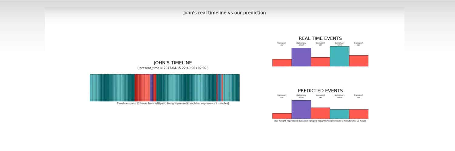
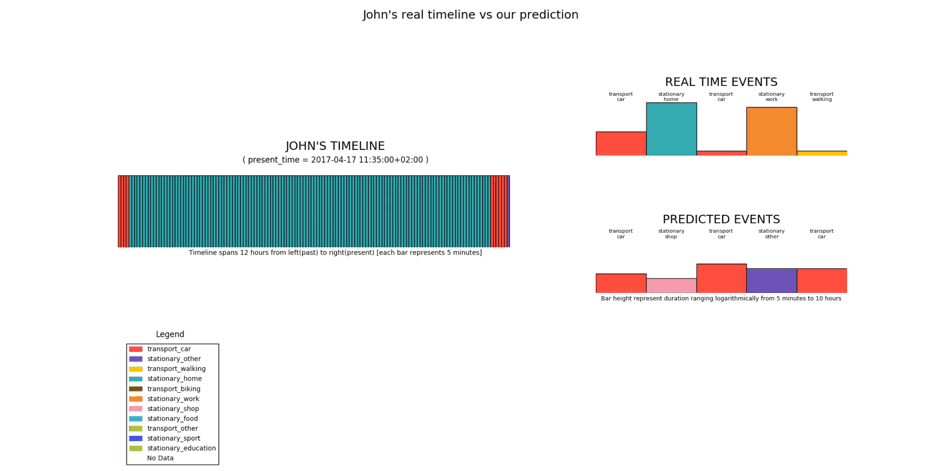
The input to our prediction model is an event timeline such as:

The figure below illustrates a simple version of a real user’s timeline with a very regular lifestyle that serves as input to the prediction model. Note that daily home/work commutes and weekend periods are clearly recognizable at first sight already in this case.
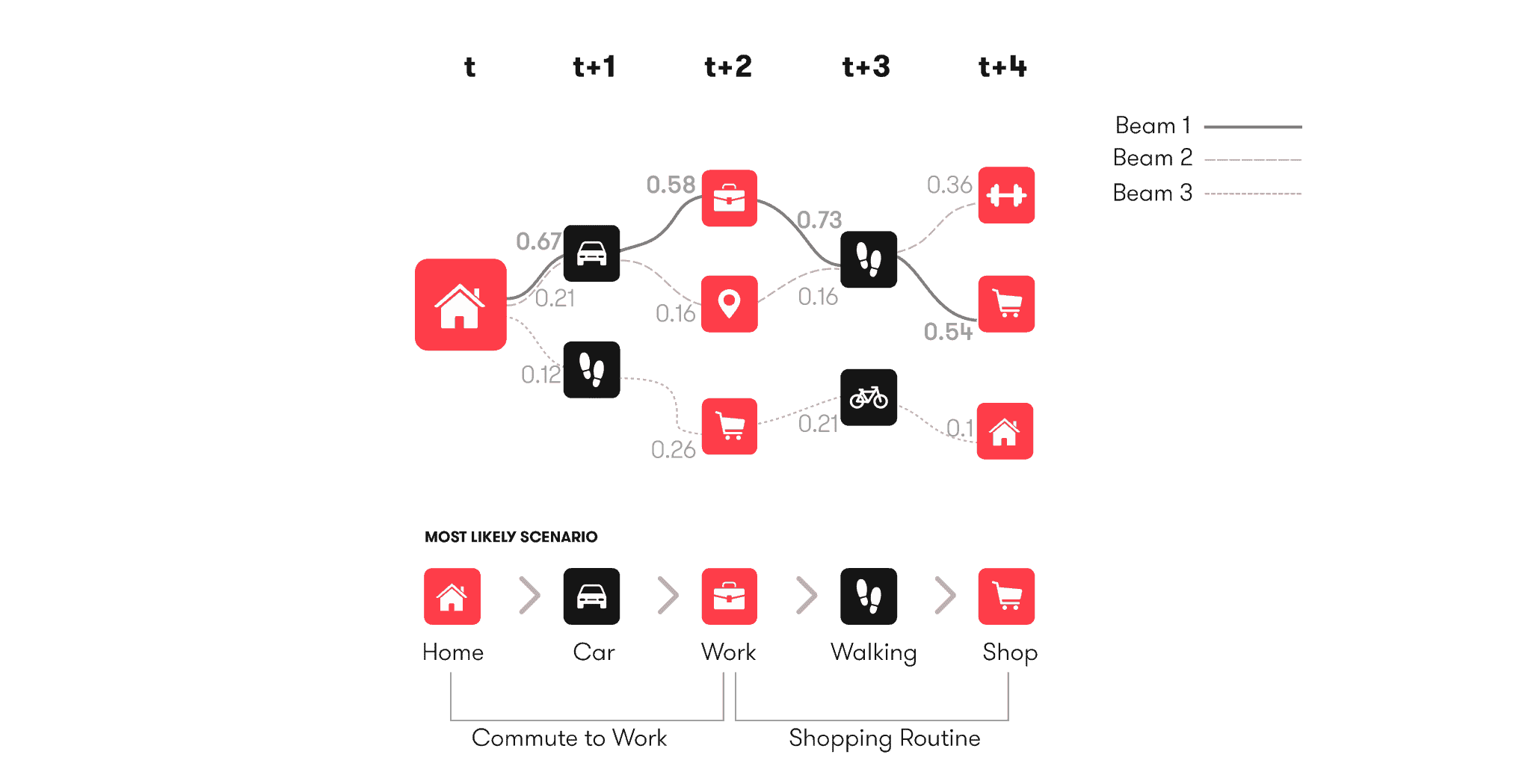
To foresee not only what a person will be doing, but also why he will be doing it, we need to be able to predict several events ahead. Consider the following example:
In order to explain the intent of the predicted ‘car’ event, our model needs to be able to understand what is likely to happen further in the future. For example:
Based on the current and future events, we can now safely assume that the underlying intent of the predicted ‘car’ event will in fact be ‘commute to work’. So predicting further ahead in time allows us to assign meaning to both current and predicted events. These semantics are what we call moments, examples of which are ‘shopping routine’, ‘commute to work’, ‘children drop-off’, ‘business trip’, ‘holiday’, and more.
Our first attempt to solve the prediction problem boiled down to a simple Markov Chain like approach where we modeled a sequence of events as:
![]()
The problem with this approach however, is that it is limited by the Markov assumption stating that the conditional probability distribution of future states only depends on the current state. As a result, this model often yields inconsistent and unlikely event predictions such as:

Thus, the network fails to learn that a person that arrives at work by bike, is also likely to leave work by bike in the evening. To avoid this kind of behavior, we would like to condition our likelihoods on all past observations, basically modeling the following joint probability:
![]()
Simply increasing the order of the Markov Chain or Bayesian network to achieve this would quickly lead to overfitting. Instead, we want our model to automatically figure out which longer-term dependencies matter and which don’t.
This is where Long Short-Term Memory (LSTM) recurrent neural networks come in. A great in-depth explanation of how LSTM works is available here. In short, LSTMs allow the neural network to automatically learn which long-term patterns are important to remember, and which are ok to be forgotten quickly.
We trained an LSTM network to learn to predict both the next event type, and the duration of the current event. This allows us to determine what the person is going to do next, and when this is likely to happen. By training a single model based on several thousands of real-world user timelines, the network learns to encode general human behavior, thereby enforcing temporal consistency at prediction time.
Moreover, using a beam-search approach, popular in NLP related literature, we are able to predict complete future timelines instead of only the next event. By retaining only the top-k most likely beams, we end up with several prediction hypotheses:
MODEL ARCHITECTURE AND TRAINING
The following figure illustrates our model architecture:
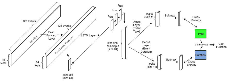
The input of the network consists of 128 previous events, each of which is represented by a feature vector that encodes the event type (e.g. ‘shop’), the day of week and time of day, and the duration of the event. A simplified example of such a feature vector is illustrated below:
This feature vector is fed into a dense input layer which basically learns to encode this information into an embedding that can be fed into the LSTM layer. The LSTM layer itself serves as an encoder: After feeding the entire sequence of events through the layer one by one, the final LSTM state encodes both the user’s general behavior and its most recent events.
The final LSTM state is then fed into a fully connected output layer which transforms the timeline encoding into a representation that is useful for actual classification.
Two different classifiers are trained simultaneously and end-to-end:
- Event type classifier (green box): What will the user be doing next?
- Event duration classifier (blue box): When will the next event start?
The event type softmax outputs 11 probabilities corresponding to the supported output types:
The event duration classifier outputs 11 probabilities corresponding to a bucketed representation of duration. The predicted duration is the expected duration of the current event and hence the start time of the next event, while the predicted event type is the expected event type of the next event.
Event durations are bucketed on a log-scale, allowing a fine-grained resolution for short events while a coarser granularity is used for longer events.
Posing the duration estimation as a classification problem instead of a regression problem greatly simplifies the global loss function that combines the duration estimation loss and the event type loss. Cross-entropy is used as the cost for both classification problems, and the final loss function is defined as the sum of both cross entropies.
Finally, we perform data augmentation to increase the model’s generalization capabilities by randomly offsetting event start and end timestamps while selecting mini batches, and by adding random noise to the event durations.
The whole network is trained on tens of thousands of real-life timelines from users with different age, gender, demographics and socio-economic backgrounds. This allows the network to generalize and to learn about typical human behavior.
RESULTS AND EXAMPLES
The following figures illustrate the confusion matrices for event type and event duration:
Clearly, some event types such as ‘Home’ and ‘Work’ are easier to predict than others, such as ‘shop’. However, note that our ground truth itself is not labeled manually and thus contains mistakes. In fact, manual inspection of the prediction results shows cases where our venue mapping fails to identify a shop or sport location correctly, while the prediction model did correctly predict the venue type. Obviously this opens opportunities for future research, where our prediction model might also be useful in a de-noising setting to clean up venue mapping or activity detection errors that happen early on in our machine learning pipeline.
Also note that the network automatically discovered that transports and venue visits are very different types of events. For example, while ‘walking’ is sometimes mispredicted as ‘car’ – mostly because walking sessions before and after parking the car are usually very short and are not always picked up by our SDK – the network almost never mis-predicts walking as ‘shop’ or ‘work’.
The duration confusion matrix shows that longer duration, represented by larger buckets, are classified correctly more often than shorter duration. Indeed, walking sessions of up to 10 minutes have quite a large variance and are often predicted to be a few minutes shorter or longer than what is observed.
An interesting observation is that jointly training the network to learn about event types and event durations improved the overall accuracy when compared to learning only about event types or event durations individually. Given the noisy ground truth data when it comes to event types, the event duration labels seems to stabilize the learning process and acts as a regularizer.
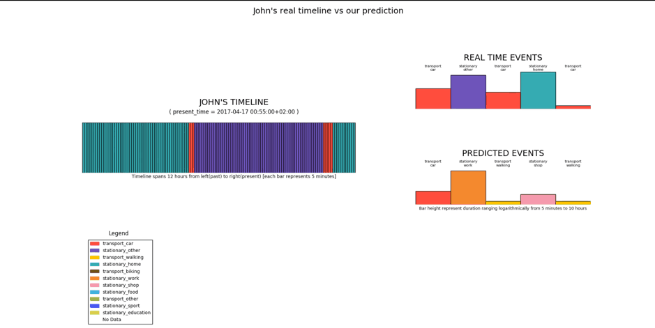
The following video illustrates some prediction results on a real-life timeline:
In the situation above, the network infers that, given the user was at home, the most likely next events are car or walking. The right-most section of the figure, containing two columns represent the different event-types (left) and the softmax-probability associated to them (right). The timeline is placed on the topmost row in the figure, and is represented as a list of 128 events, each event having a different color, as listed in the legend.
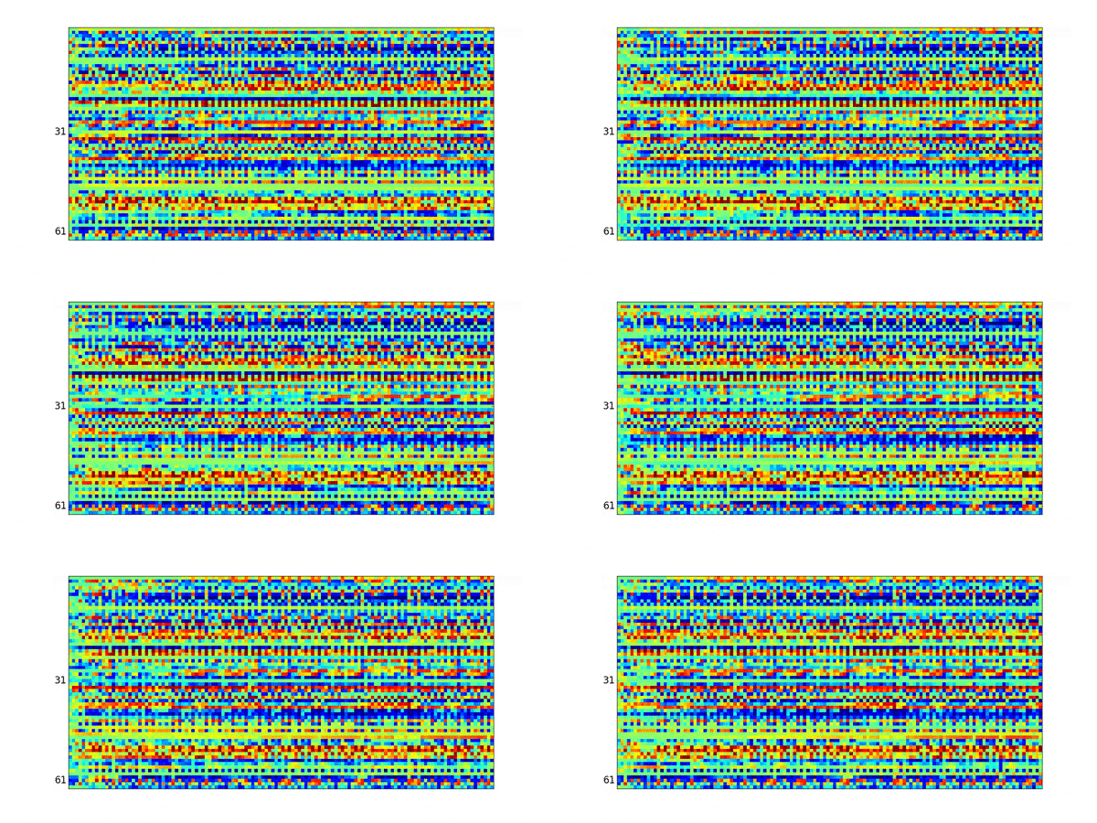
Below the timeline, are drawn the different internal state and gate values for the LSTM cells, in the form of separate panels. Each of the state and gate panels are 128X64 matrices in the above image, where 128 is the length of the timeline, and 64 is the size of an LSTM cell used in the model.
Now let’s zoom into the LSTM States plot:
Among the 64 LSTM cell units (rows of this 128X64 matrix) we can clearly distinguish between (i) those that have learned to depend only on local input features, and (ii)those that have learned to remember and recognize temporal patterns in the sequence of inputs. For instance if we take a closer look at row number 61 in the above matrix:
We see that the LSTM cell units simply translate from right to left, almost entirely retaining their state values. This implies that these units have only learnt the features specific to the event they are tied to and have not learnt any temporal patterns, because if they did so, their values would change as the sequence progressed in time. On the other hand, if we look at row number 31 in the same LSTM state matrix:
As the units translate from right to left, their value keeps changing in this case and as a whole, there appears to be smooth variations across the stretch of the entire row-sequence. Two inferences are to be drawn: (i) the smooth variations in the LSTM cell units’ state values show signs of coordinations between temporally consecutive cell units, i.e. cell units in a close temporal neighborhood behave similarly which intuitively appears to be an equivalent of a self-learned convolutional kernel (with subsequent max-pooling), and (ii) the only way of explaining the variations in LSTM cell unit state values here is that the units do learn temporal patterns apart from the features of the event they are tied to, and that is why they keep changing values as the sequence progresses in time. More interestingly, in the above sample, the leftmost units which are more than 100 events back in the past still keep changing their values, which implies that the network is able to learn long term dependencies spanning over 100 events in some cases (like the one above).
Whereas rows 61 and 31 are the two extreme cases (of local and temporal patterns respectively), the behavior in the other rows is definitely somewhere in between. The ability to learn long-term dependencies often allows the network to predict event types in cases where even human observers would have difficulty to correctly predict the correct event.
For example, we noticed cases where the network knew that a user was going to sport at a time at which the user normally does not sport, simply by recognizing the sequence of events and event durations that led up to the current moment. By examining the user’s general past behavior, and by closely monitoring the sequence of events and event durations that led up to the current moment, the network is able to predict the unexpected. Clearly this kind of behavior can not be accomplished by simple Bayesian approaches modeling ![]()
PREDICTING FAR AHEAD
Simply predicting the next event type and current event duration is useful in cases in which we engage with the user at the right time. However, for more complicated use cases that require estimates of intent (e.g. ‘commute to work’ or ‘shopping routine’), we need to be able to predict several events ahead.
Moreover, we want to predict several hypothesis timelines, such that we can quickly adapt our future predictions if the next event turns out to be different from what we predicted.
To accomplish this, we use a beam-search approach, which traverses a search tree of prediction hypotheses and retains only those sequences that maximize the total log likelihood:
Below is a video that illustrates the beam search based predictions for a sample user:
The actual event that happened after Home, was Car, which is among the predictions suggested (i.e. Car or Walking). Given that the next event was Car, the model now predicts that the next event is going to be Stationary_Other, which as shown below, happens to be a correct prediction.
The above scenario uses real user data and the predictions are made over the Easter-weekend time-period. Weekends are usually difficult to predict, but it is evident that in general, the model is close enough at predicting the sequence of future events. It has inherently learnt the meaningful transitions between stationary events and transport events. And has also learnt the duration that a particular event type usually spans over (walking means short time, home means long, etc.). However, there is a special scenario here, which is the Easter Monday (a holiday in Belgium). If we notice at the instance shown below, the model on Sunday night thinks that the next day is a work day, when it actually is not.
It makes sense for the model to think so, because after all, an Easter Monday happens rarely enough to be considered an anomaly. However, the good part is that on the next day, as soon as the user goes to a place which is not his/her workplace, the model immediately adapts itself to predict further events in the future as if it was not a typical working day, but a weekend-ish day with shopping and other events. This displays the dynamic adaptability that our new prediction model possesses.
Apart from the above weekend example, below is a video showing predictions for a weekday routine, where the predictions look more correct (as expected, because weekdays are more predictable on average):
CONCLUSION
Based on our state-of-the-art machine learning and sensor fusion pipelines part 1 and part 2 Sentiance offers the most accurate event detection and contextualization capabilities on the market today.
Our deep learning based prediction pipeline adds extremely precise predictions to our solution, allowing our customers to engage with their users at the right time. Moreover, being able to predict several events ahead, allows us to model intent, thereby explaining why a user will be performing a specific action.
Do you want to enrich your customer experience and deliver personalized and context-aware engagement? Reach out to us.

