Introduction

At Sentiance, we developed a platform that takes in smartphone sensor data such as accelerometer, gyroscope and location information, and extracts behavioral insights. Our AI platform learns about the user’s patterns and is able to predict and explain why and when things happen, allowing our customers to coach their users and engage with them in the right way, at the right time.

An important component of our platform is the venue mapping algorithm. The goal of the venue mapper is to figure out what venue you are visiting, given an often inaccurate location measurement coming from the smartphone’s location subsystem.

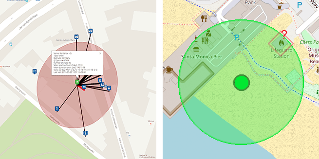
Figure 1: Left: Venue mapping means estimating which of the neighboring venues a user was actually visiting.
Right: Human intuition helps us to quickly discard unlikely venues, such as the lifeguard station when a user is visiting the beach.

Although venue mapping is a difficult problem altogether and will be material for a future blog post, a simple sense of human intuition based on the surrounding geography of the area often goes a long way. Consider the example of a visit to the Santa Monica State Beach illustrated by figure 1. The chance that this user is actually visiting the lifeguard station is probably rather small, given a glance at the immediate surroundings.

Indeed, simply by looking at a map of the area, humans are often able to quickly discard unlikely venues and to formulate a prior belief on what is actually happening. Is the venue located in an industrial area, a park, nearby the beach, in a city center, our nearby a highway?

To equip our venue mapping algorithm with the same sense of intuition, we developed a deep learning based solution that is trained to encode geo-spatial relations and semantic similarities describing a location’s surroundings. This is illustrated conceptually by figure 2.

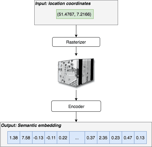
Figure 2: The area surrounding a given location is rasterized and passed to a deep neural network. This network acts as an encoder, outputting an embedding that captures the high level semantics of the input location.

The encoder transforms locations into distributed representations, similar to what Word2Vec [1] does for natural language. These embeddings reside in a metric space and therefore adhere to the rules of algebra. Using word embeddings for example, we can reason about word similarity and analogy. We can even perform arithmetic operations such as “king - man + woman = queen” directly in the embedding space.

In the next few paragraphs we will discuss how we designed a solution that learned to map location coordinates into a metric space that allows us to do similar things, as illustrated by figure 3.

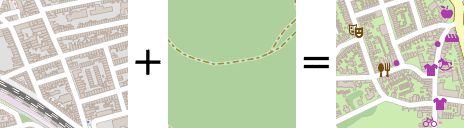
Figure 3: The proposed solution directly optimizes a metric space, such that basic arithmetic operations can be used to explore the embedding space.

Tile generation

Rasterizing GIS data

Given a location coordinate and a radius, we can query our GIS database to obtain a large amount of geographical information. Our GIS database is a local copy of OpenStreetMap stored in a PostGis database. PostGis is a convenient PostgreSQL extension that adds support for spatial operators, types and indices.

For example, using a set of queries, we can easily check if there is a river nearby a location fix, what the distance is to the nearest train station, and whether or not the location is nearby a road. Moreover, the actual road itself can be fetched as a polyline, while the outlines of the train station building might be available as a polygon object.

However, it is unclear how this large amount of unstructured data can be presented efficiently to a neural network for further processing. Taking into account our goal of training a neural network that understands about shapes and spatial relations such as distance, inclusion, occlusion, and exclusion, we decided to rasterize a location’s surroundings to a fixed size image before feeding it into the encoder.

Luckily, efficient tools are available to do exactly that. We coupled Mapnik and its Python bindings with a customized version of the OpenStreetmap-Carto stylesheets, resulting in a fast rasterizer that we can use to generate image tiles, as shown by figure 4.

Figure 4: Mapnik is used to rasterize GIS data fetched from PostGis into an image.

We parameterized our rasterization service to easily do data augmentation by rotating and shifting the map before generating the image tile. This is illustrated by figure 5, where image patches representing the same location are shown with different orientation angles and horizontal and vertical offset values.

Figure 5: Our tile generator allows for easy data augmentation by rotating and shifting the map before generating an image tile.

From image to tensor

Although these rasterized image tiles would allow our encoder to easily learn to capture spatial structures and relationships, a lot of information is lost during rasterization. In fact, rasterization merges all polygons and polylines such as roads, buildings, park outlines, rivers, etc. Since our GIS database contains information on each of these structures separately, it does not make sense to require the neural network encoder to learn to segment them.

Instead of rasterizing the data into a three-channel RGB image, as illustrated above, we, therefore, modified the rasterizer to produce a 12-channel tensor, where each channel contains the rasterized information of a different type. Figure 6 shows such a 12-channel tensor for the same coordinates as used in figure 5.

Figure 6: A 12-channel tensor is used to represent the area. Each channel contains specific information, such as road networks, land cover, amenities, etc.

For easy visual interpretation, we will often show the RGB rasterized version instead of the 12-channel tensor in the remainder of this article.

Representation learning

Spatial similarity

Our goal is to learn a metric space where two semantically similar image patches correspond to two embedding vectors that are close together. The question then becomes how to define ‘semantically similar’.

A naive approach to obtain a similarity space could be to represent each image patch with its histogram, use k-means clustering, and model the space using a bag of words model. However, it is unclear which channels should be assigned what kind of weights. For example, if the roads are similar, but the buildings are not, then are the two patches still semantically similar?

Moreover, even if two patches have a similar histogram, this does not tell us anything about the spatial structures of the location surrounding. If half of an image patch is covered by ocean, then is this patch semantically similar to a patch that contains a lot of small ponds, lakes or fountains? Figure 8 shows two image patches that yield almost identical histograms:

Figure 7: Histogram based clustering does not suffice to capture semantic similarities and spatial relations. These two images have almost identical histograms, while their semantic meaning is quite different.

However, these image patches are not semantically identical. The first patch covers an area of interconnecting roads, while the second patch covers some small roads that probably lead to people’s homes. Indeed in our embedding space, we find that the Euclidean distance between the embeddings of both patches is quite substantial ($|p_1-p_2|_2=2.3$) even though the Chi-Square distance between their histograms is close to zero.

Apart from using histograms, each channel could be summarized by a set of features such as histograms of oriented gradients or more traditional SIFT or SURF descriptors to capture spatial relations. However, instead of trying to manually specify which features define semantic similarity, we decided to use the power of deep learning to learn to detect meaningful features automatically.

To accomplish this, we feed the 12-channel tensor into a convolutional neural network that acts as our encoder. The network is trained using a triplet loss function in a self-supervised manner, meaning that no manually labeled data is needed during training.

Self-supervised learning: Triplet networks

The triplet loss concept, inspired by siamese network architectures, was proposed by Ailon et al. [2] as a means to perform deep metric learning for unsupervised feature learning.

A triplet network is a neural network architecture that is trained using triplets $(x, x^+, x^-)$ consisting of:

• An anchor instance $x$
• A positive instance $x^+$ that is semantically similar to $x$
• A negative instance $x^-$ that is semantically different from $x$

The network is then trained to learn an embedding function $f(.)$, such that $| f(x) - f(x^+) |_2 < | f(x) - f(x^-) |_2$ and thus directly optimizes a metric space. This is illustrated by figure 8.

Figure 8: Triplet networks are trained using a triplet loss such that a metric space is learned where similar instances are close to each other, while dissimilar instances are far away from each other.

Metric learning using a triplet network was popularized further by Google's FaceNet [3], where a triplet-loss is used to learn an embedding space for face images, such that embeddings of similar faces are close to each other, while those of different faces are far away from each other.

For face recognition, positive images are pictures from the same person as the anchor image, while negative images are pictures from a randomly selected people in the mini batch. In our case, however, we don’t have classes from which we can easily select positive and negative instances.

To define semantic similarity we can make use of Tobler’s first law of geography: “Everything is related to everything else, but near things are more related than distant things”.

In the following, let $I(.)$ be a mapping from location coordinates to a rasterized image patch. Given a transformation $T(.)$ that rotates and shifts the map before rasterizing an image patch for location $X$, and given a random location $Y$ such that $X neq Y$, we can obtain our triplets as:

• $x = I( X )$
• $x^+ = I( T(X) )$
• $x^- = I( Y )$

We thus assume that two geographically nearby, partially overlapping patches are semantically more related than two completely different image patches. Figure 9 shows two examples of such triplets, both with the same anchor image.

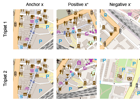
Figure 9: Triplets consist of an anchor image, a positive image, and a negative image.

To keep the neural network from learning only trivial transformations, we also randomly enable or disable some of the 12 channels for each positive instance during training. This forces the network to consider a positive patch to be similar to an anchor patch even if a random subset of the information is different (e.g. no buildings, no roads, etc.).

SoftPN triplet-loss function

Figure 10 illustrates the general structure of our triplet network.

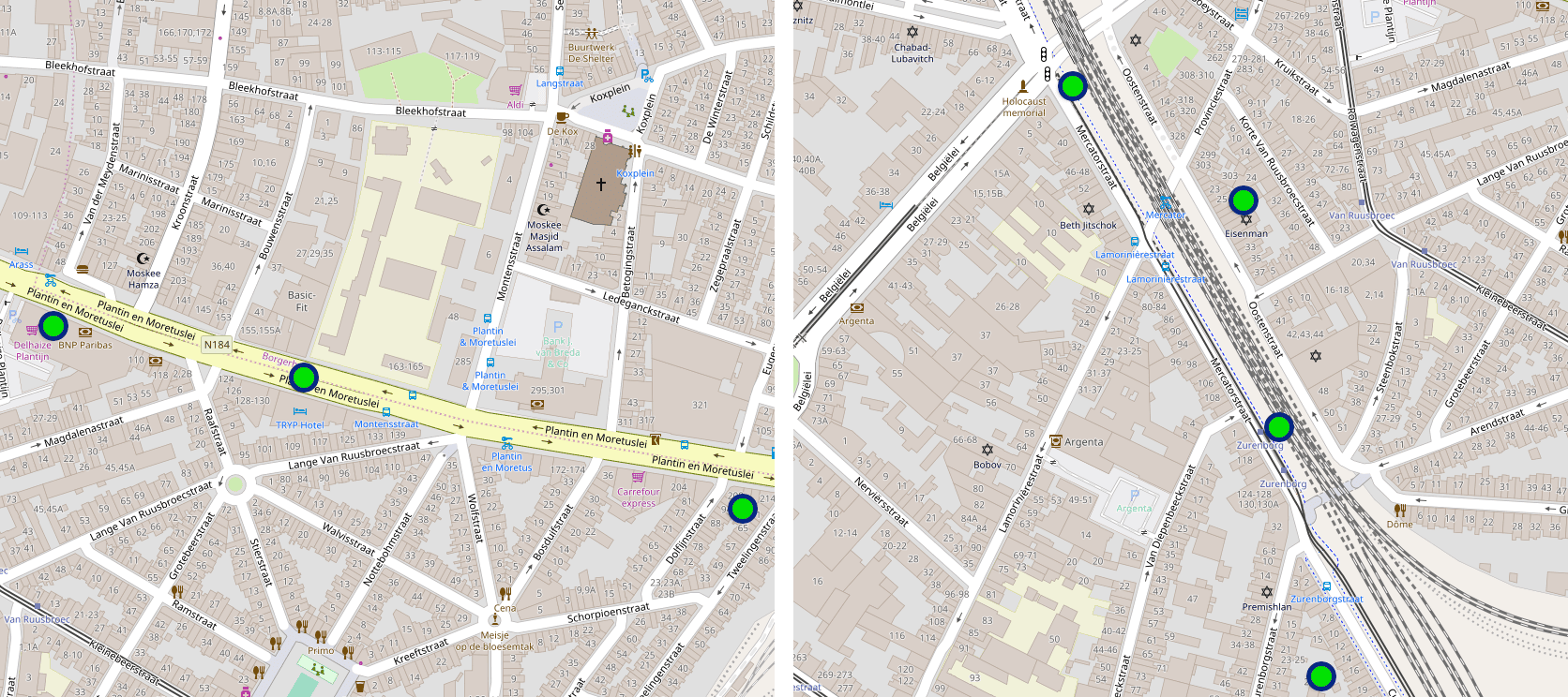
Figure 10: The triplet loss directly optimizes the ratio of the distance between anchor and positive embeddings, and the distance between anchor and negative embeddings.

The loss function is defined as $Loss(d_+, d_-) = Delta((d_+ - 0), (d_- - 1))^2$ so that optimizing the network corresponds to minimizing the MSE of the vector $(d_+, d_-)$ compared to the vector $(0, 1)$.

To see why the loss function is defined this way, consider that we want $Delta(a, p)$ to be as close to zero as possible, while we want $Delta(a, n)$ to be as large as possible. To optimize this ratio, a SoftMax is applied to both distances to obtain bounded similarities in the domain $[0, 1]$:

$d_+ = frac{e^{Delta(a,p)}}{e^{Delta(a,p)} + e^{Delta(a,n)}}$ , $d_- = frac{e^{Delta(a,n)}}{e^{Delta(a,p)} + e^{Delta(a,n)}}$

This definition of the triplet-loss is often referred to as the SoftMax ratio and was proposed originally by Ailon et al. [2].

The main problem with this definition is that it is very easy for the network to quickly learn an embedding space where $d_-$ is close to one, simply because most random negative images radically differ from the anchor image. As a result, the majority of $(a, n)$ pairs do not contribute a lot to the gradients in the optimization process, causing the network to quickly stop learning.

To solve this, different approaches can be used, one of which is hard-negative mining [3] which boils down to carefully selecting $(a, n)$ pairs to make sure the network keeps learning. However, in our case, it is not always clear how to efficiently select hard-negatives without introducing bias into the learning process. A simpler solution, is the use of the SoftPN triplet-loss function, proposed by Balntas et al [4].

The SoftPN loss replaces $Delta(a,n)$ in the above SoftMax calculation with $min(Delta(a,n), Delta(p,n))$. The effect is that during optimization, the network tries to learn a metric space where both the anchor and the positive embeddings are as distant as possible from the negative embedding. In contrast, the original SoftMax ratio loss only considered the distance between the anchor and the negative. This difference is illustrated by figure 11.

Figure 11: The SoftPN loss optimizes the more difficult problem by maximizing the minimum distance between negative instance and either anchor or positive.

Neural network architecture

As an encoder we used a fairly traditional convolutional neural network architecture containing 5 convolutional layers with filter size 3x3, followed by two layers with 1D convolutions and a densely connected layer. One dimensional convolutions are used to reduce the dimensionality towards the top of the network by means of cross-channel parametric pooling [5].

The embedding layer itself is made up of another dense layer with a linear activation function such that the output does not stay limited to the positive domain after the non-linearity of the previous layer. The complete network architecture is illustrated in figure 12.

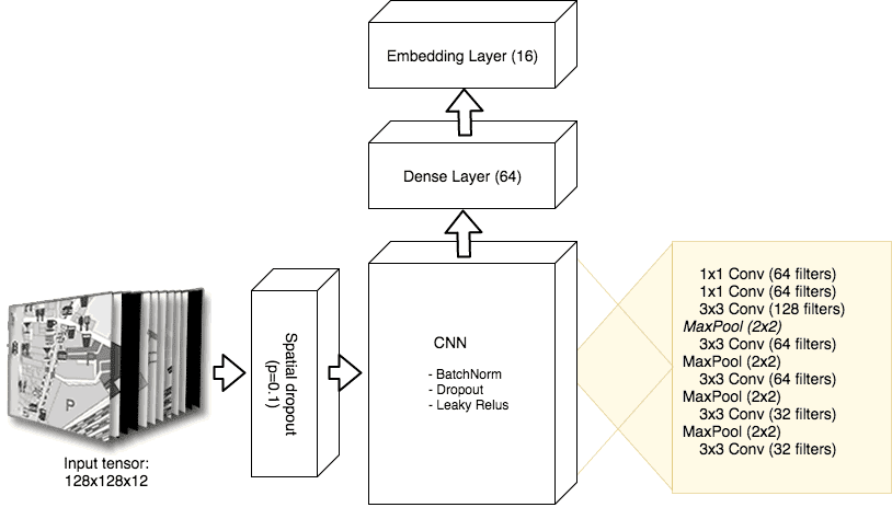
Figure 12: The encoder comprises of a convolutional neural network, followed by a fully connected layer. The final embedding layer is a dense layer with a linear activation function.

We aggressively make use of dropout and batch-normalization, and use Leaky Relu activation functions to resolve the problem of dying Relus that was observed during initial test runs.

Additionally, spatial dropout is applied directly to the input. This causes a randomly selected input channel to be completely dropped, forcing the network to learn to distinguish images by focussing on different channels.

The complete network, implemented using Keras, only contains 305,040 parameters and was trained for two weeks on a p3.2xlarge AWS machine using the Adam optimizer.

Training data

To generate our training data, we fetched about 1 million locations that were visited by users on our platform and added approximately 500,000 location fixes that were captured while users where in transport.

For each of those 1.5 million locations, we rasterized an image tile of size 128x128x12, representing an area around the location with a radius of 100 meters. These tensors served as anchor images.

For each location, we also rasterized 20 randomly shifted and rotated image tiles which served as negative images. The offset was uniformly sampled between 0 and 80 meters in both horizontal and vertical directions. This results in 20 (anchor, positive) pairs for each location, and 30 million images in total.

Triplets were generated on the fly while generating a mini batch during network training. Each mini batch contained 20 locations. For each location, we randomly selected 5 (anchor, positive) pairs to have a meaningful representation of the anchor-positive distances. Negative images were selected randomly within each mini batch, resulting in a total minibatch size of 100.

Generating mini-batches of triplets on the fly virtually results in an almost infinitely large dataset of unique triplets, encouraging the network to keep learning for many epochs.

Visualizing filters and activations

As the embedding space is learned in a self-supervised manner, without labeled data, it is difficult to monitor whether or not the network is actually learning anything during training.

An insufficient but still useful check is to visualize the filters learned by the network. In fact, we would like to visualize input images that maximize the activations of different layers in the network.

To do this, we can start with a randomly generated image, and consider each pixel to be a parameter to be optimized. We then update the image pixels using gradient ascent such that it maximizes the output of a chosen layer.

Computing the gradient of the input image with respect to the mean output activation of the convolutional layer and running gradient ascent for a few iterations, yields images that highlight the structures that are of most interest to the layer.

Since our input is a 12-channel tensor, not an RGB image, we simply select three of the 12 channels with the highest mean pixel magnitude and arrange these into an RGB image. We apply histogram equalization to each channel to further enhance the visual details.

Figure 13 shows the results of each of the 32 filters of one of the bottom layers of the network. Clearly, this layer seems to focus on low-level details such as roads and small blob structures.

Figure 13: The bottom layers of the network learn to detect low-level details such as roads and small blob-like structures and icons.

Figure 14 visualizes the 64 filters of one of the upper layers. These filters clearly get activated more by smoother and more complicated structures, which indicates that the network indeed might be learning a hierarchical feature decomposition of its input.

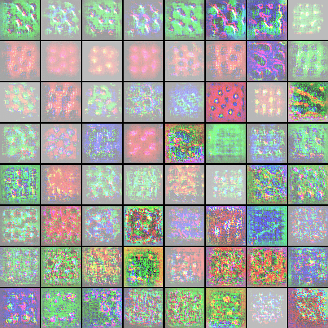
Figure 14: The upper layers of the network tend to learn more complicated structures by combining low-level features from lower layers.

Although the usefulness of these visualizations should not be overestimated, they are fun to look at, especially during the many research iterations. For example, early versions quickly pointed us into the right direction to discovering a bunch of dead Relus in our network. This was subsequently solved by replacing these with leaky Relu activation functions.

Exploring the metric space

Visualizing the embeddings

Visualizing the filters learned by the network is mostly interesting while debugging the network but does not help a lot in judging the quality of the learned embedding space.

To get a sense of how the embedding space looks like, figure 15 instead shows the embedding space after using PCA to reduce the dimensionality to 3D. Each location embedding is visualized by its rasterized image tile for ease of interpretation.

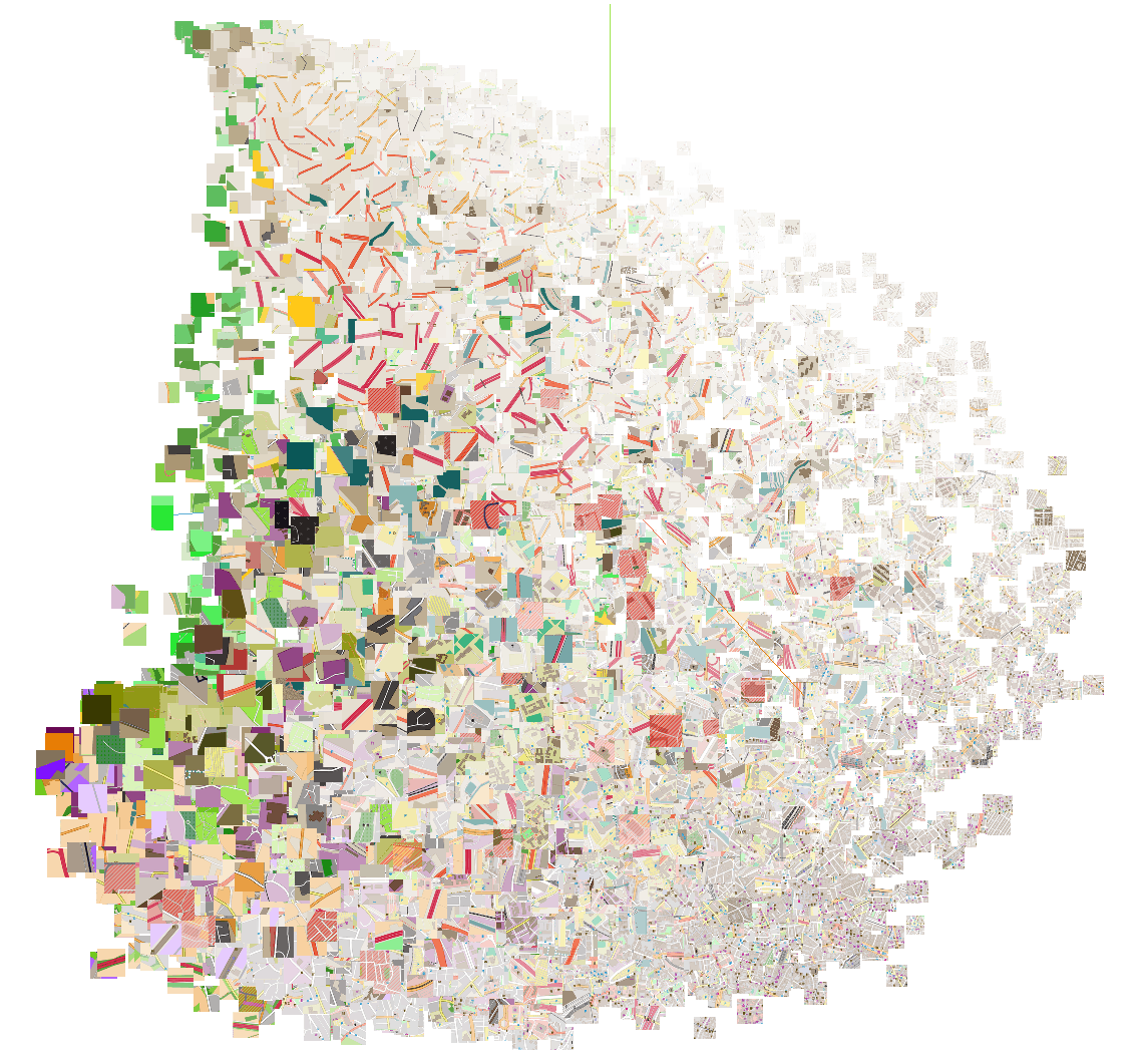
Figure 15: 3D plot of the embedding space obtained by means of PCA.

This clearly shows that even just the first three principal components capture a lot of interesting information. Green areas such as parks are clearly distinguishable from the different road types such as highways and primary roads, and from the city centers in the right-bottom corner of the plot.

To more clearly show these local structures, figure 16 shows an animation of a 3D t-SNE plot of the embedding space.

Figure 16: 3D plot of the embedding space obtained by means of t-SNE.

Although venue mapping is one clear use case of these embeddings, they can also be used by our transport classifier. Figure 17 shows a scatter plot of embeddings of location fixes that were fetched from our transport classification training set. In this case, Linear Discriminant Analysis (LDA) was used to project the 16-dimensional embedding space to 2D.

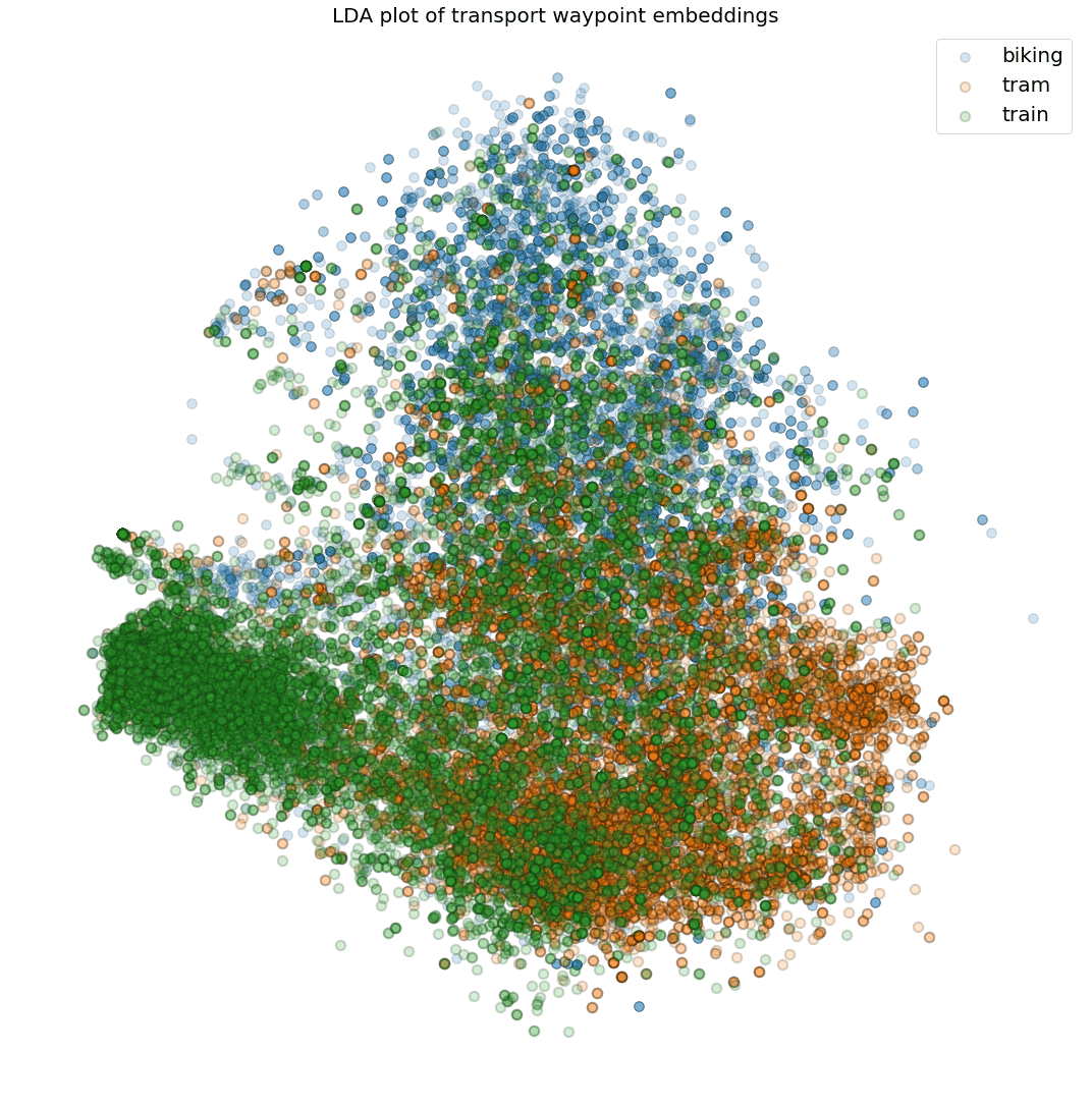
Figure 17: 2D LDA plot of the embedding space for waypoints gathered during transport sessions.

This plot shows that different transport modes generally occur in different areas. For example, our embeddings capture information about train tracks or tram stops.

To show how different geographical areas are encoded, we used PCA to reduce the 16D embeddings to 3D, which were scaled and used directly as RGB color values to plot our test dataset on a map. This is illustrated in figure 18, where we zoomed in on the city of London, UK. The figure clearly shows that city centers, highways, water areas, tourist areas and residential areas are encoded differently.

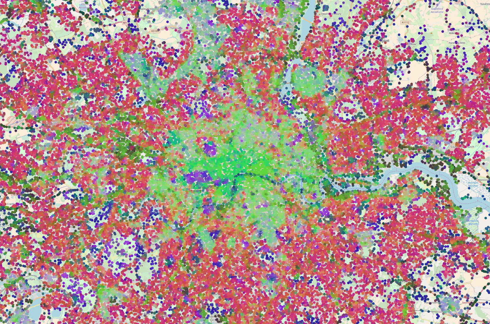
Figure 18: Embeddings for randomly sampled locations in London, UK. The color is obtained by using PCA to reduce the 16D embedding vectors to 3D RGB triplets. (Click to enlarge)

Doing a similar trick for the city of Birmingham, UK, reveals a larger suburban area compared to London, while the area surrounding London contains a lot more buildings. This is illustrated in figure 19.

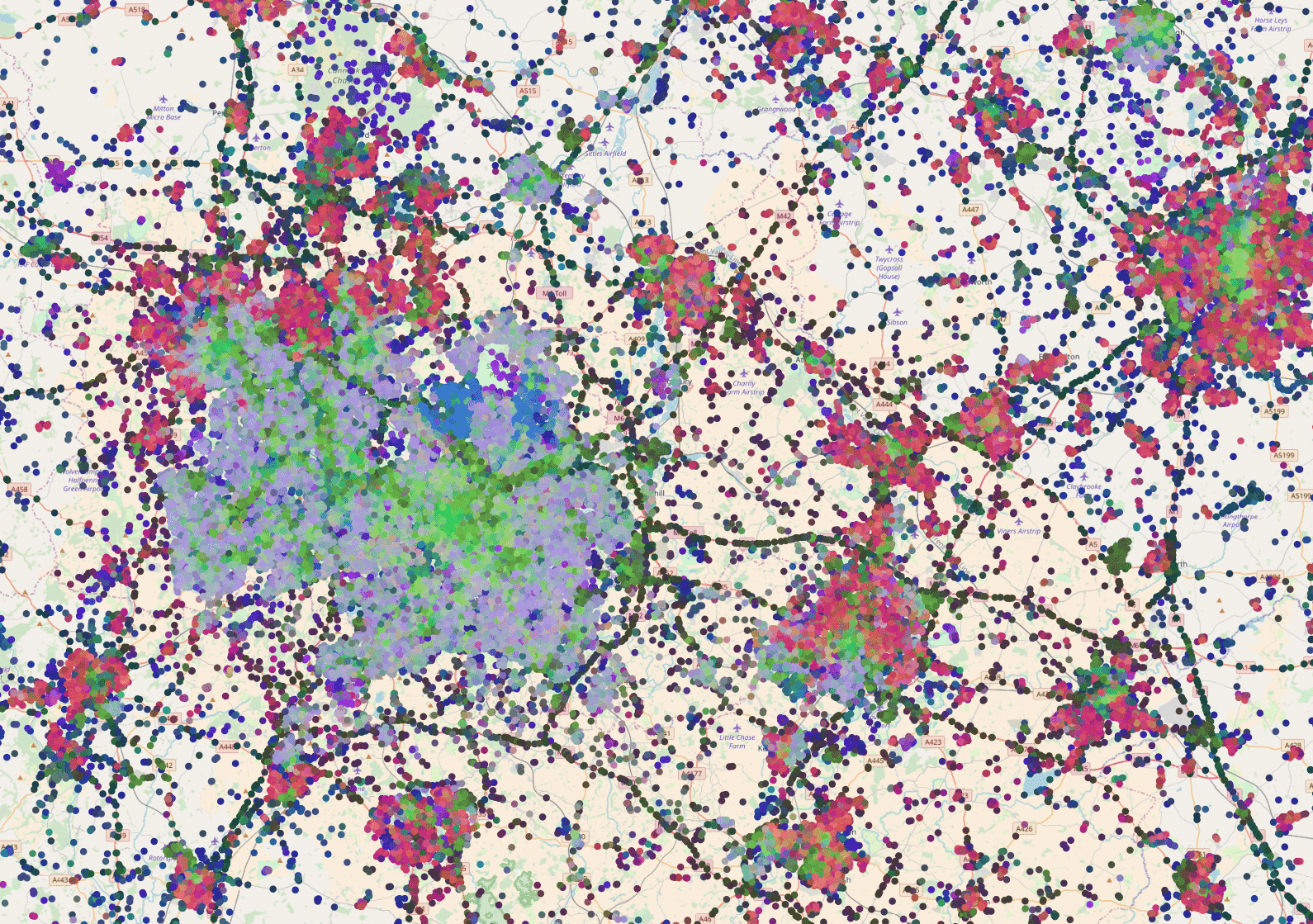
Figure 19: Embeddings for randomly sampled locations in Birmingham, UK. The color is obtained by using PCA to reduce the 16D embedding vectors to 3D RGB triplets. (Click to enlarge)

A random walk through space

To further examine the smoothness of the embedding space, we can do random walks, starting from a random seed point. At each jump, we randomly select one of the k-nearest-neighbors of the current embedding and visualize the corresponding image patch.

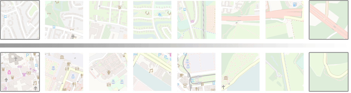
Figure 20 shows the result of several such random walks. Note that most of the time, nearest neighbors in embedding space are hundreds or thousands kilometers away from each other geographically speaking, but have a high semantic similarity.

Figure 20: Six random walks through the embedding space, each time starting from a different seed point.

Calculating with locations

While the above visualizations indicate that the learned embedding space is smooth and learned to capture semantic similarity, it does not prove that we actually learned a Euclidean metric space. In such a space we should be able to interpolate between embeddings and perform basic arithmetic operations while getting meaningful results.

Figure 21 illustrates the result of interpolating between two embeddings, from left to right. At each step during interpolation, the resulting embedding is mapped to the nearest embedding in our test data, and the corresponding image tile is visualized.

Figure 21: Interpolation from one embedding (left) to another (right), while showing nearest neighbor images from our test data at each intermediate step.

Finally, figure 22 shows what happens when we start adding or subtracting embeddings, and mapping the result to the nearest neighbor in our test data.

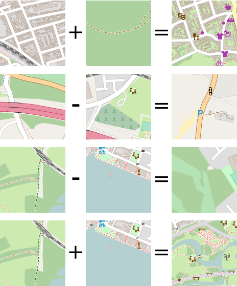
Figure 22: Calculating with embeddings, and mapping the result back to the nearest neighbor image in our test data.

These results indicate that our embedding space indeed represents a metric space in which distance has meaning and the rules of a basic arithmetic hold.

Since this metric space is trained in a self-supervised manner, huge amounts of unlabeled data can be used to force the network to learn to capture meaningful relations. Using these embeddings as feature vectors in our subsequent classifiers, therefore, corresponds to a form of transfer learning, allowing us to train powerful classifiers with very limited amounts of labeled data.

Conclusion

In this article, we showed how a triplet network can be used to learn a metric space that captures semantic similarity between different geographical location coordinates.

A convolutional neural network was trained to learn to extract features that define this semantic similarity, and an embedding space was obtained by means of metric learning.

The resulting embedding space can be used directly for tasks such as venue mapping or transport classification and helped us to greatly improve our classifier accuracies and generalization capabilities by means of transfer learning.

Moreover, these embeddings add a sense of intuition to our classifiers such that incorrect classifications still make intuitive sense. For example, the venue mapper quickly learns to tie day and night time activities to specific areas such as industry zones, city centers, parks, train stations, etc.

If you want to learn more about our platform or try it out yourself, don’t hesitate to contact our sales team, or download our demo app: Journeys!

References

[1] Mikolov, Tomas, et al. "Efficient estimation of word representations in vector space." arXiv preprint arXiv:1301.3781 (2013).
[2] Hoffer, Elad, and Nir Ailon. "Deep metric learning using triplet network." International Workshop on Similarity-Based Pattern Recognition. Springer, Cham, 2015.
[3] Schroff, Florian, Dmitry Kalenichenko, and James Philbin. "Facenet: A unified embedding for face recognition and clustering." Proceedings of the IEEE conference on computer vision and pattern recognition. 2015.
[4] Balntas, Vassileios, et al. "PN-Net: Conjoined triple deep network for learning local image descriptors." arXiv preprint arXiv:1601.05030 (2016).
[5] Lin, Min, Qiang Chen, and Shuicheng Yan. "Network in network." arXiv preprint arXiv:1312.4400 (2013).