Introduction
At Sentiance, we developed an AI platform that learns to detect and predict a person's behavior, routines and profile from mobile sensor data such as accelerometer, gyroscope and GPS. Many low level algorithms, such as our transport mode detector, are trained by supervised learning techniques for which we gathered labeled data by closely collaborating with our partners, customers and test groups. However, supervised learning comes with at least two major drawbacks:
- Gathering labeled data in a natural setting can be difficult and very expensive.
- The algorithm does not improve over time, even when millions of unlabeled data points per day are captured.
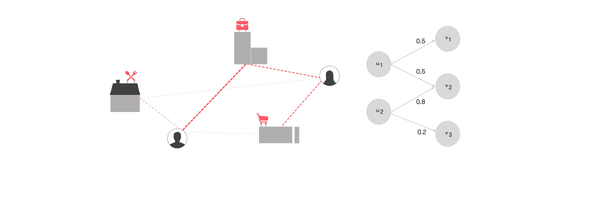
A concrete example that would benefit from unsupervised or semi-supervised learning, is venue mapping, i.e. figuring out which venue a user is visiting given a noisy location estimate. Since the type of place a user is currently visiting highly depends on his recent and long-term past behavior, this kind of data needs to be gathered in a realistic setting where the temporal behavior of the user actually corresponds to natural human behavior. While gathering labeled data for venue mapping is a tedious process, getting unlabeled data comes for free as more users are using our platform. The question then becomes: Can we extract meaningful information from population-wide human visiting patterns without requiring access to the actual labels?
The main motivation for this project is therefore to enable us to learn from these large unlabeled datasets, with minimal preprocessing and feature engineering. More specifically, we want to learn a representation of a location that embeds different types of meaningful information, for example the category (e.g. shop, school, etc.) of the place present at that location, and some information about population-wide behavior at that location. We can then use these representations in our venue mapping and other models.
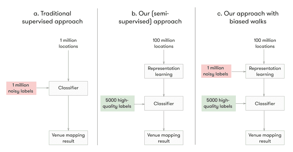
To achieve this, we adapt the DeepCity deep learning framework (Pang, 2017), which is inspired on word2vec word embeddings (Mikolov, 2013) and graph embeddings (Perozzi, 2014).
DeepCity
DeepCity (Pang, 2017) is a feature learning framework based on deep learning, to profile users and locations. It uses check-in data obtained from online social networks such as Facebook, Twitter, Foursquare, etc. Users frequently share their whereabouts using those platforms in the form of so-called check-ins. Two use cases are considered: user profiling, and location profiling. In the context of user profiling, it is assumed that the whereabouts of a user reflects who he or she is. User profiling includes tasks such as age or gender prediction and is the focus of Pang et al. Location profiling, on the other hand, is aimed at learning more about locations and includes tasks such as predicting the category of a location. The latter is the focus of this blog, because of the direct link to venue mapping.
User and location profiling tasks are being handled by machine learning algorithms, typically involving hand-engineered features. The latter is very time consuming and requires domain-specific knowledge. Even with expert domain knowledge, it is difficult to capture all relevant features, that are applicable in all scenarios. Deep learning provides a promising alternative, where features are no longer hand engineered but are learned by the model itself. DeepCity (Pang, 2017) can be considered such an approach, specifically for user and location profiling.
DeepCity uses a graph representation of check-ins and random walks on this graph and outputs node embeddings. More specifically, location and user nodes are organized in a bipartite graph, and task-specific random walks are used to explore the graph. Using those random walks and some clever algorithms we can learn our embeddings. But let’s take a step back first, and put everything into context.
From word embeddings to graph embeddings
DeepCity (Pang, 2017) is based on graph or network embeddings (Perozzi, 2014) using the skip-gram model (Mikolov, 2013). The objective is to learn representations (embeddings) that preserve each user’s or location’s neighbor information. We then use these embeddings as features for other models (e.g., user or location profiling). In addition, we can fine tune these representations to specific tasks. Manual engineered features are no longer needed.
To understand the type of graph embeddings proposed in the DeepCity paper we first need to go back to natural language processing, more specifically the word2vec and the skip-gram model (Mikolov, 2013). The goal of the word2vec algorithm is to learn a representation for each word given a corpus. It became known and popular due to interesting properties, such as the ability to do arithmetics with them. A famous example:
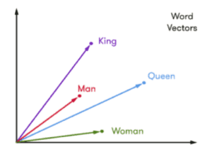
Figure 1: Word vector examples for ‘king’, ‘man’, ‘queen’, and ‘woman’.
The word2vec algorithm has also been adapted to graphs, for example in the context of social networks. DeepWalk (Perozzi, 2014), among others, uses word2vec in the context of graphs: graph nodes correspond to words, and random walks on the graph are used to generate the sentences. Below is an example from the DeepWalk paper (Perozzi, 2014). The input (left) is the famous Zachary’s karate club graph where nodes are assigned a label (color), and the outputs (right) are the node embeddings. The embeddings capture the structure and labels of the network. More recently related approaches have started to show up in the specific context of location based social networks (Pang, 2017).

Figure 2: (left) Zachary’s Karate Club Graph, and (right) DeepWalk representation. Image Source: DeepWalk paper (Perozzi, 2014)
Graph representation of check-ins
Graph construction
Similar to the DeepWalk algorithm (Perozzi, 2014) described above, DeepCity (Pang, 2017) uses a graph representation and random walks, and outputs node embeddings. More specifically, locations and users are organised in a bipartite graph based, and (task-specific) random walks are used to explore the graph.
The input to the DeepCity algorithm consists of (timestamp, user id, venue id) check-in records. From those check-ins, we can construct a bipartite graph, that links users and the venues they visit. Let’s consider a small example check-in dataset. The dataset consists of two users that work in the same office. One of the users typically gets lunch at a nearby supermarket, whereas the other user often brings lunch but sometimes gets a sandwich.
| User | Venue | Check-ins | Description |
|---|---|---|---|
| u1 | v1 | 5 | Supermarket |
| u1 | v2 | 5 | Office |
| u2 | v2 | 4 | Office |
| u2 | v3 | 1 | Sandwich Shop |
We can represent the check-in dataset as a bipartite graph, linking users and visited venues.
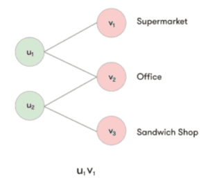
Figure 3: Example (unweighted) bipartite check-in graph.
We assign weights to the edges of the bipartite graph, e.g., based on the visit frequency, and obtain a weighted bipartite graph. We introduce the notation $latex u in U$ to denote a user, and the notation $latex v in V$ to denote a venue. We denote the bipartite graph between the set of users $latex U$ and the set of venues $latex V$ by $latex G = (U, V, W_{V, U})$ where $latex W_{V, U}$ represents the weighted edges between locations and users. We define $latex c_v$ to be the total number of check-ins at venue $latex v$, and $latex c_u$ the total number of check-ins by user $latex u$, and $latex c_{v, u}$ as the number of check-ins by user $latex u$ at venue $latex v$.
We then define the edge weight from $latex u$ to $latex v$, and from $latex v$ to $latex u$ as:
$latex w_{u, v} = frac{c_{v, u}}{c_u}$, and $latex w_{v, u} = frac{c_{v, u}}{c_v}$
We obtain the following edge weights for the earlier example:

Figure 4: (left) Example (unweighted) bipartite check-in graph, (center) weighted check-in graph (users → venues), (right) weighted check-in graph (venues → users).
Random walks
Now that we have a graph representation of the visits, where the graph nodes can be considered words in word2vec sense. We now need a way to generate sentences from this graph representation. For this, we use random walks. At each node in the random walk, we randomly sample one of the neighbors based on the edge weight. Below is an example random walk sequence.[/vc_column_text]
| Step | Random Walk Sequence |
|---|---|
| 0 | u1 → v1 |
| 1 | u1 → v1 → u1 |
| 2 | u1 → v1 → u1 → v2 |
| 3 | u1 → v1 → u1 → v2 → u2 |
| 4 | u1 → v1 → u1 → v2 → u2 → v3 |
We can now assume that the graph nodes (temporal users and venues) correspond to words, and that the random walks correspond to sentences. We can now apply the word2vec algorithm (Mikolov, 2013) to the random walk sequences and obtain embeddings of the graph nodes. However, the authors of the DeepCity paper actually go one step further and propose task-specific (or biased) random walks, which we will consider next.
The DeepCity framework (Pang, 2017) uses task-specific random walks, which use location and user properties to guide the feature learning to be more specific to each task. In other words, the random walks are guided towards certain users or locations which are more relevant to the prediction task in mind.
To achieve this, a measurement to quantify to which extent a user is biased towards location categories is proposed. We can determine the check-in distribution of the population over the location categories, and for each user. A user is assumed to be biased when his or her check-in category distribution P is different from the population check-in category distribution Q. The authors propose the Kullback-Leibler divergence to define such a bias: KL(Q|| P). As a result, users who exhibit behavior similar to that of the whole population get low bias values, whereas users with different behavior get higher bias values.
Assume a category bias value $latex x_{u, category}$ for user $latex u$, we then obtain the category biased edge weight from venue $latex v$ to user $latex u$:
$latex w^{category}_{v,u} = w_{v, u} , x_{u, {category}}$
The edge weight from user to venue remains unchanged. The underlying idea is that we want to visit more interesting users more often in the random walks and see what other places they visit. We show an example below of a check-in category distribution of the population (left) and example user (right).
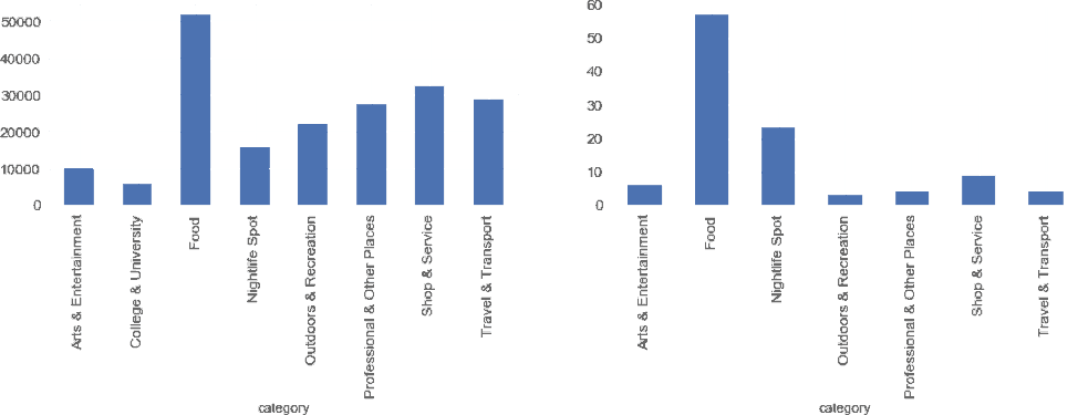
Figure 5: (left) Population, (right) Example user
Note that in order to perform task-specific random walks we need labeled data, i.e., we need to be able to associate a category with each venue. If users check-in to specific venues (e.g., using online social networks), this is easily obtained, however when only a (latitude, longitude) pair is available, like in our situation, this is no longer the case and we need some way to approximate this information in order to use task-specific walks. We will discuss such modifications later, but first, we will have a look at some experimental results.
DeepCity for labeled data
Experimental Setup
For the purpose of this blog post we used the TSMC2014 NYC check-in dataset (Yang, 2014) for all research experiments. The dataset consists of about 10 months of check-in data in New-York and was collected from Foursquare between April 2012 and February 2013. Each anonymized user in the dataset has at least 100 check-ins, but a venue may have only a single check-in.
We present the dataset statistics of the raw dataset and those of the filtered dataset used in the experiments. In addition, we also include the statistics of the dataset used in the DeepCity paper (Pang, 2017), although they can not be compared due to different data collection procedures, filtering, etc. We filtered the NYC dataset (Yang, 2014) by requiring at least 10 check-ins at each venue, which is in line of the experiments in (Pang, 2017), and by removing certain categories, for example, those with a temporary nature such as events, or without a fixed location.[/vc_column_text]
| Raw | Filtered | DeepCity | |
|---|---|---|---|
| Venues | 38.333 | 34.937 | 54.961 |
| Check-ins | 227.428 | 194.258 | 19.600.207 |
| Users | 1.083 | 1.083 | 1.165.286 |
| Active users | / | / | 12.778 |
We trained 128-dimensional embeddings over 50 epochs using a linear decreasing learning rate. During an epoch, a random walk of length 100 is generated for each venue and temporal user node. We use the skip-gram architecture with negative sampling (5 negative samples) and a context window of size 11.
A logistic regression classifier is used for the location profiling task, i.e., given a venue embedding predict the corresponding venue category. We used 5-fold cross-validation and report the average results over the folds. Grid search was used to determine the optimal hyper-parameters (e.g., regularization).
Exploring DeepCity Embeddings
Let’s start by taking a look at the learned embeddings before we start building other models on top of them. Below we show a 2D representation of the embeddings obtained by applying the T-SNE algorithm. We colored each venue node according to its category, and are able to discover structure in it, which we highlighted.
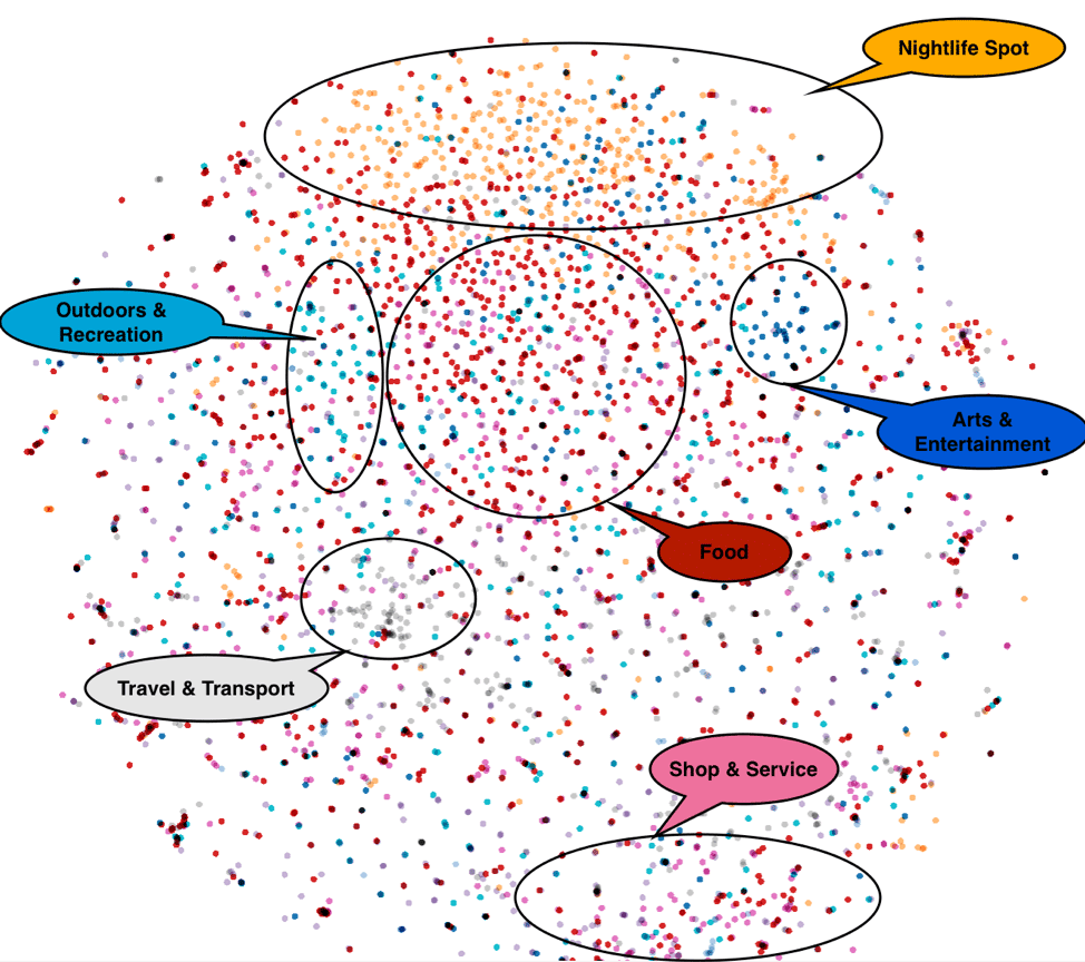
Figure 6: DeepCity venue embeddings visualized using t-SNE. Venue nodes are colored according to their venue category.
Let’s see how subcategories are organized. We now consider the Travel & Transport category and corresponding subcategories. In the PCA based representations below we filtered on this category, and highlight a specific subcategory.
Notice for example that Hotels (left) are grouped together in one part of the space, and airport-related venues (right) are grouped together in another part of the space.
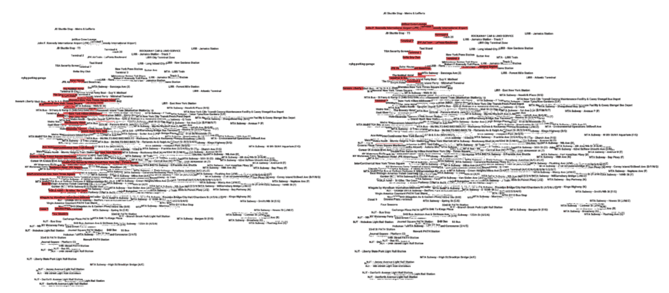
Figure 7: DeepCity travel & transport venue embeddings visualized using PCA. (Left): Travel & Transport (white), Hotels (red). (Right) Travel & Transport (white), Airport (red)
We can also take a look at the different transport modes used in New York, and again we notice that they are grouped together in somewhat distinct areas of the space, e.g., metro in the left figure, bus in the right figure.
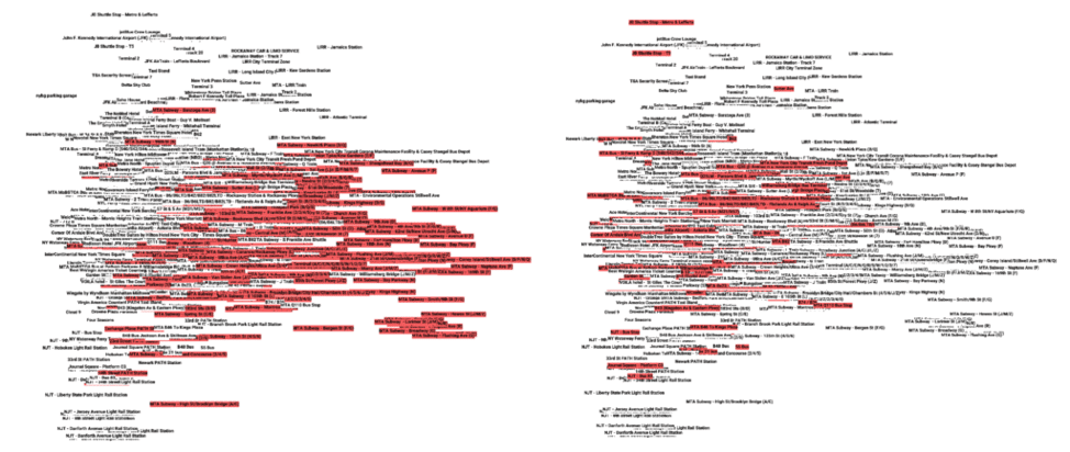
Figure 8: DeepCity travel & transport venue embeddings visualised using PCA. (Left): Travel & Transport (white), Subway (red). (Right) Travel & Transport (white), Bus (red)
Word embeddings, such as those obtained from the word2vec algorithm described earlier, are based on the distributional hypothesis: “You shall know a word by the company it keeps” (Firth, 1957). A similar idea exists in the context of geography, and is called Tobler’s first law of geography: “Everything is related to everything else, but near things are more related than distant things.” (Tobler, 1969). Let’s explore these ideas a bit further. The venues are this time colored according to their postal code. Notice that the embeddings capture the geospatial relations, i.e., nodes with the same color cluster together.
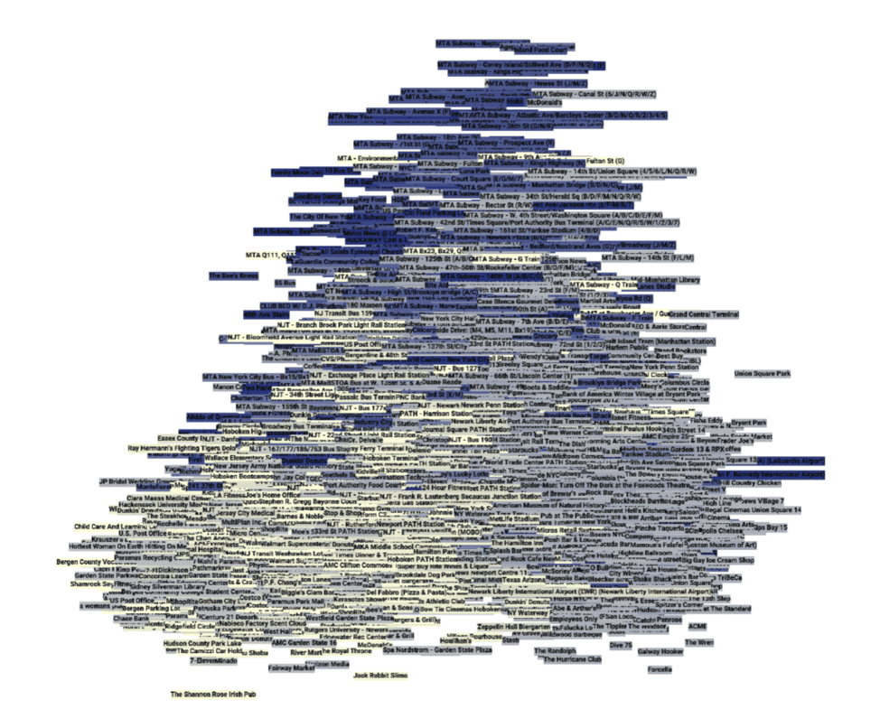
Figure 9: DeepCity travel & transport venue embeddings visualized using PCA. Venue embeddings colored according to postal code.
These visualizations show that the resulting embeddings capture both geo-spatial distance and semantic similarity at the same time, distributed over different dimensions of the embedding vector.
Given a certain venue as query point, we can also easily determine the nearest neighbors in the embedding space. Let’s determine the five nearest neighbors for some example venues.
| Venue | Category | Distance |
|---|---|---|
| Terminal 3 | Travel & Transport | 0.460 |
| JetBlue Crew Lounge | Travel & Transport | 0.478 |
| Jb Shuttle Stop - T5 | Travel & Transport | 0.486 |
| Delta Sky Club | Travel & Transport | 0.503 |
| JB Shuttle Stop - Metry & Lefferts | Travel & Transport | 0.538 |
| Query: John F. Kennedy International Airport (Travel & Transport) | ||
Notice that the query results are all related to travel and transport, even though there are other types of venues located in the same airport, that are also present in our dataset. This again shows that both geography and semantic similarity are capture simultaneously.
Let’s consider another example, but this time related to related arts and entertainment.
| Venue | Category | Distance |
|---|---|---|
| The Metropolitan Area | Arts & Entertainment | 0.248 |
| The Joyce Theater | Arts & Entertainment | 0.272 |
| Elinor Bunin Munroe Film Center | Arts & Entertainment | 0.291 |
| BAM Harvey Theater | Arts & Entertainment | 0.317 |
| Brooklyn Sports Club | Outdoor & Recreation | 0.328 |
| Query: Carnegie Hall (Arts & Entertainment) | ||
Again, the the nearest neighbours are also related to arts and entertainment, but there is one somewhat unexpected venue present. Let’s consider a final example related to nightlife.
| Venue | Category | Distance |
|---|---|---|
| PH-D at Dream Downtown | Nightlife Spot | 0.369 |
| Mother's ruin | Nightlife Spot | 0.380 |
| Wharf Bar & Grill | Nightlife Spot | 0.408 |
| Electric Room | Nightlife Spot | 0.412 |
| Top of the Standard | Nightlife Spot | 0.417 |
| Query: Le Bain (Nightlife Spot) | ||
From these initial observations, we already get indications that the Deepcity framework embeds meaningful information for location profiling purposes, such as categories, subcategories, and geospatial information.
Location Profiling
Let us now consider the location profiling task, our main interest. Given a location embedding, we want to predict the category associated with this location. Before presenting our results, let us first consider the results presented in (Pang, 2017), using their custom NYC dataset.
| Micro-F1 | Macro-F1 | Weighted-F1 | |
|---|---|---|---|
| Unbiased | 51.00% | 33.00% | / |
| Biased | 63.00% | 48.00% | / |
| Reference results (Pang, 2017) | |||
Below are the results using the TSMC2014 NYC dataset (Yang, 2014). We include the results from a few trivial classifiers to help putting the results in context
- Most frequent: always predict the most frequent category in the dataset.
- Uniform: sample uniformly from the categories.
- Stratified: sample from the categories based on the distribution present in the dataset.
| Micro-F1 | Macro-F1 | Weighted-F1 | |
|---|---|---|---|
| Most Frequent | 28.03% | 5.47% | 12.27% |
| Uniform | 11.39% | 10.54% | 12.42% |
| Stratified | 16.65% | 12.40% | 16.58% |
| Unbiased | 38.06% | 35.81% | 37.56% |
| Biased | 41.24% | 39.09% | 41.15% |
| Sentiance results | |||
Although we are using a similar type of dataset (i.e., Foursquare check-ins in NYC), our results are not as good as reported in the paper (Pang, 2017). However, we do observe a similar influence of the type of random walks. Although the results are not ideal (i.e., we would have preferred the same or better scores) they still demonstrate the potential of the method.
Sparse Labels
In the DeepWalk paper (Perozzi, 2014) the authors considered the scenario of sparsely labeled training data, i.e., only a limited amount of (node) labels are available. This is interesting because we do have a limited amount of labeled data that we can use. We, therefore, experimented with sparse labels in the context of the DeepCity framework (Pang, 2017).
We first learned embeddings using the regular (unbiased) random walks and task-specific (biased) random walks. We then trained a classifier that predicts the category given an embedding. We kept the test set fixed, but trained the classifier using increasing amounts of data.
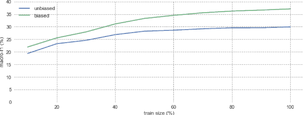
Figure 10: Evaluation of location profiling performance in function of the amount of training data.
We obtain the best results when all available training data is used, but the approach is also promising when only a limited amount of data is available.
Extending DeepCity to unlabeled datasets
General approach and initial results
Until now we have considered the DeepCity framework (Pang, 2017) in the context of (labeled) check-in datasets, where we know the exact venue or place that is being visited. We must adapt the framework in order to support our (unlabeled) stationary datasets. The difference between the two types of data is shown in the table below.
| Type | Data | Data Collection |
|---|---|---|
| Stationary |
|
Implicit (By our SDK) |
| Check-in |
|
Explicit (By manual user action) |
We first needed to move from an infinite amount of often noisy (latitude,longitude) pairs, to a discrete set of locations or places. Clustering algorithms may come to mind, but would add additional complexity. What we need is a simple and deterministic way to map (latitude, longitude) coordinates to a discrete set of locations. Geohashes are therefore an ideal candidate, which represent latitude and longitude information as a string, where the precision depends on the number of characters used.
We now have the minimum requirements for the DeepCity framework (Pang, 2017): check-in tuples (user, timestamp, place). However, at this point we can only use unbiased random walks, which are not tuned to the specific task under consideration (e.g., location profiling). In order to support task specific (biased) random walks, we need contextual data (labels).
We need contextual information for two purposes. First we need contextual data for task-specific walks. Second, we need ground truth contextual information to evaluate the embeddings in the location profiling task, i.e., category prediction. Check-in datasets from location based social networks do include this type of information, but as mentioned before, we do not always have access to such ground truth data. Can we make an informed guess on the category to assign to a certain geohash (area)?
The basic idea is to consult a point-of-interest provider to find nearby venues and pick the most common category among those venues. Clearly, this is a very crude approximation, but it is trivial to implement. Of course, we could use more elaborate approaches, but we intentionally kept things as simple as possible. We consider two point-of-interest providers or views:
- Check-in view: We extract venues from the check-in dataself itself. Consequently, we will only be aware of venues for which check-ins were observed during the data collection period. Note that other venues may exist in the area, but those are unobserved. In other words, this view is related to what the users actually do.
Micro-F1 Macro-F1 Weighted-F1 Most Frequent 31.08% 5.93% 14.74% Uniform 11.40% 9.94% 13.26% Stratified 20.44% 12.19% 20.33% Unbiased 33.81% 29.04% 34.87% Biased 38.16% 32.14% 38.82% Sentiance results: Check-in View - Infrastructure view: We obtain venues directly from the point-of-interest provider, which will contain the unobserved venues that are missing in the check-ins view. In other words, this view is related to which venues are located in the area, which does not necessarily reflect what users actually do.
Micro-F1 Macro-F1 Weighted-F1 Most Frequent 40.41% 7.20% 23.26% Uniform 11.69% 9.30% 14.18% Stratified 27.27% 12.81% 26.95% Unbiased 27.27% 19.74% 29.88% Biased 31.47% 21.20% 33.95% Sentiance results: Infrastructure View
Influence of noisy labels
To evaluate the impact of noise introduced by the place and context approximations we consider the following scenarios:
Scenario 1:
- Train embeddings using the infrastructure view.
- Train classifier using the check-ins view.
- Evaluate classifier using the check-ins view.
Scenario 2:
- Train embeddings using the infrastructure view.
- Train classifier using the infrastructure view.
- Evaluate classifier using the check-ins view.
The motivation behind scenario 1 is to evaluate if it is possible to learn task-specific embeddings from a large but noisy dataset, but train and evaluate them on a less noisy location profiling task. For example, we could learn the embeddings on a large scale unlabeled dataset, and train and evaluate a location profiling model using a smaller labeled subset of that dataset. In this scenario, we consider a “best case” giving us an upper limit, because we use all data.
The motivation of scenario 2 is to evaluate the impact of noisy training data (i.e., approximations of the category associated with a location) on the embeddings learnt by the DeepCity framework and the location profiling model. Let’s take a look at the results obtained in both scenarios.
| Micro-F1 | Macro-F1 | Weighted-F1 | |
|---|---|---|---|
| Most Frequent | 31.08% | 5.93% | 14.74% |
| Uniform | 11.44% | 9.94% | 13.26% |
| Stratified | 20.44% | 12.19% | 20.33% |
| Unbiased | 34.20% | 29.10% | 34.83% |
| Biased | 35.05% | 26.76% | 34.17% |
| Sentiance results: Scenario 1 | |||
| Micro-F1 | Macro-F1 | Weighted-F1 | |
|---|---|---|---|
| Most Frequent | 25.13% | 5.02% | 10.10% |
| Uniform | 12.49% | 10.83% | 14.47% |
| Stratified | 17.36% | 9.84% | 15.40% |
| Unbiased | 21.68% | 19.96% | 21.21% |
| Biased | 21.90% | 19.05% | 20.49% |
| Sentiance results: Scenario 2 | |||
The main conclusion from Scenario 1 and 2 is that biasing the random walks does not help when the biases are determined using noisy training data (labels). Let’s take a closer look at the different “views” used in the experiments.
In this section we will consider the following:
- What is the influence of the views on the location category distribution?
- How much “conflicts” arise?
- What is the influence on the bias values?
Below is the distribution of categories considering different “views” on the data. We want to compare which type of places are visited at a certain location, versus what type of places is present at that location according to our venues database. There is quite some difference between the different views.
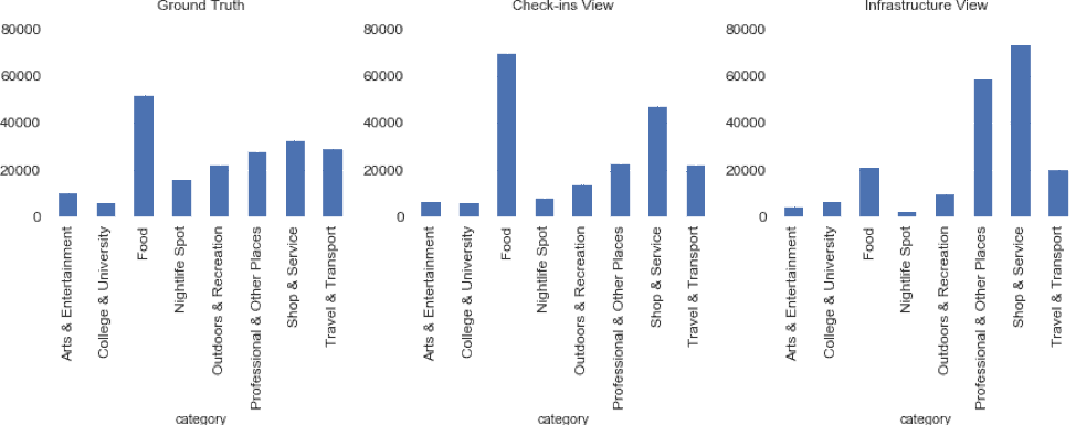
Figure 11: Distribution of categories using different “views” on the data.
As mentioned before, because geohashes are used, it can happen that one geohash corresponds to one or more venues, possibly with different categories. The following graph gives us an idea of the “confusion” typically seen. In general, there is only a single venue category that is being actively checked-in to in a given geohash.
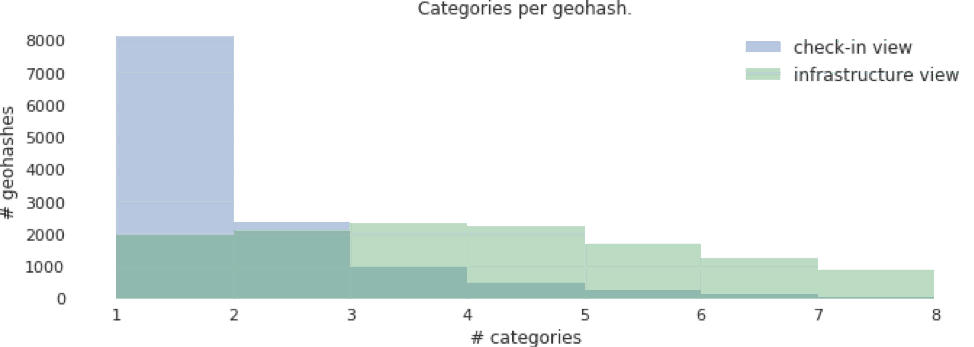
Figure 12: Number of distinct categories per geohash.
Finally, let’s take a closer look at the bias values used in the different experiments. The “approximate” views (checkins view and infrastructure view) are similar, but they are quite different from the biases used in the ground truth case, which may explain why the (biased) task-specific walks no longer provide many benefits.
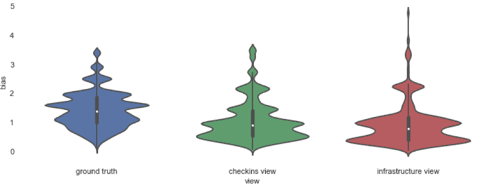
Figure 13: Violin plots of the bias values obtained using the different views.
Conclusion
We have evaluated the location profiling capabilities from the DeepCity framework (Pang, 2017) and showed that it is capable of learning representations for location profiling tasks, that capture different types of information. Task-specific random walks can be used to guide the learning algorithm to learn similarities that are more relevant to the task, for example, category prediction.
We have shown how the framework can be extended to support unlabeled datasets. However, in such a use case we must be careful with using task-specific random walks based on possibly noisy labeled data. Experiments have indicated that in a scenario with noisy training data, task-specific random walks may have a negative effect on the performance.
We also evaluated the potential of the framework when labels are sparse, which would allow hybrid approaches, where the embeddings are trained on large unlabeled datasets, and specific models that depend on them are trained using a limited amount of labeled data by benefiting from the generalization properties of these type of embeddings.
We are currently integrating DeepCity location and/or user embeddings (together with other types of embeddings) in our existing models such as the venue mapping algorithm. You can test our latest innovations yourself by installing Journeys or getting in touch with our sales team.
Every day at Sentiance is challenging and rewarding! Our team is growing fast and we are looking for talented people who want to make an impact working on game-changing technologies.
Be one of the change-makers and join our team!
References
- Tomas Mikolov, Kai Chen, Greg Corrado, Jeffrey Dean, “Efficient Estimation of Word Representations in Vector Space”, ICLR 2013 Workshop, 2013.
- Tomas Mikolov, Ilya Sutskever, Kai Chen, Greg S. Corrado, Jeff Dean, "Distributed Representations of Words and Phrases and their Compositionality", Advances in Neural Information Processing Systems 26 (NIPS 2013), 2013.
- Bryan Perozzi, Rami Al-Rfou, Steven Skiena, “DeepWalk: Online Learning of Social Representations”, Proceedings of the 20th ACM SIGKDD international conference on Knowledge discovery and data mining (KDD '14), 2014.
- Dingqi Yang, Daqing Zhang, Vincent W. Zheng, Zhiyong Yu. Modeling User Activity Preference by Leveraging User Spatial Temporal Characteristics in LBSNs. IEEE Trans. on Systems, Man, and Cybernetics: Systems, (TSMC), 45(1), 129-142, 2015.
- Jun Pang, Yang Zhang, “DeepCity: A Feature Learning Framework for Mining Location Check-ins”, Eleventh International AAAI Conference on Web and Social Media (ICWSM '17), 2017.

