From Cloud to near real-time On Device
At Sentiance we turn motion into insights, thus transport mode detection is one of our core technologies. We were using and were happy with our deep learning-based solution, deployed in the Cloud, for a long time (see - Large scale transport mode classification from mobile sensor data). Yet finally technology enables us to transition towards a more privacy-friendly and resource-efficient solution that can work on-device.
Both Android and iOS offer basic real-time on-device activity detection for transport modes (aka. motion activities). However, these are not what we actually mean by saying Transport Classifier. Instead of always flip-flopping momentary predictions, we aim to segment a trip into multi-modal blocks to understand when you are walking, running, driving, cycling, etc.

we want to segment a trip into stable transport modes (bottom).
Such transport mode classification is more valuable if we want to understand if you are a green commuter, a public transport user or a die-hard driver. In addition to that, near real-time predictions would allow us to run hyper-personalized campaigns and know - when to target a person?
In this blog post, we will share a methodology that we used to achieve near real-time Transport Classification that runs on-device and delivers stable transport mode segmentation. Compared to our current production Transport Classifier in the cloud, we managed to create an end-to-end solution that fits into TensorFlow Lite (tflite) and that replaces complex business logic block with neural network all the way.
Building blocks of a Transport Mode Classifier
As an input we want to feed raw sensor data (accelerometer, GPS fixes, GIS features, etc.) and as an output get the current transport mode. We want all signal processing, prediction and segmentation to be executed on device with as short a response time as possible. For sure there are some complications:
- there might be gaps in sensor data and the sampling rate can vary over time
- each multimodal trip has varying size and range is huge (from minutes to hours)
- Transport Classifier needs to ignore some events like phone handlings and idles
- the solution needs to stay small and have minimal impact on phone battery life and CPU
- we aim for real-time classification, but at the same time it's impossible to be confident when a new transport mode begins without waiting at least a bit (as you will soon see that bit will be around 3 minutes)
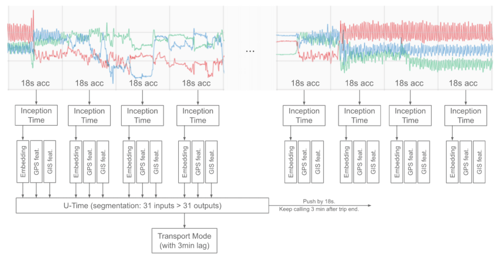
To solve these problems we will use a two-step approach that combines Inception architecture with U-net (see Figure 2 ):
- Pre-process raw accelerometer signal using approximate interpolation to take care of varying sampling rates and gaps (jump to section).
- Construct accelerometer signal embedding optimized for transport classification (jump to section). At this stage 18 seconds worth of sensor data is converted into a vector of size 8.
- Segment a trip into different transport modes using obtained embeddings (jump to section). These embeddings (spanning more than 9 minutes) enriched with GPS and GIS features are passed to the U-time inspired segmentation model to get a prediction that lags by 3 minutes.
- Bundle all blocks into a single tflite model that expects a call every 18 seconds (jump to section).
In the sections to come we will explain our design choices and discuss some implementation details.
Step 1. Approximate interpolation
To kickstart things, we know that sensor sampling rate can change and we want to apply some signal processing (at least a low-pass filter). After some research, we stumbled upon a neat idea from B. Llanas (Constructive approximate interpolation by neural networks, 2006, doi) which essentially says that there is a way to do approximate interpolation and smoothing using diffs (and sums) of values at times t.
Let (1) 
It can be interpreted quite intuitively if you think about what happens if A is huge in which case it approximates a point by a step function. Not only that, controlling the A value allows achieving a similar effect to using a low-pass filter.
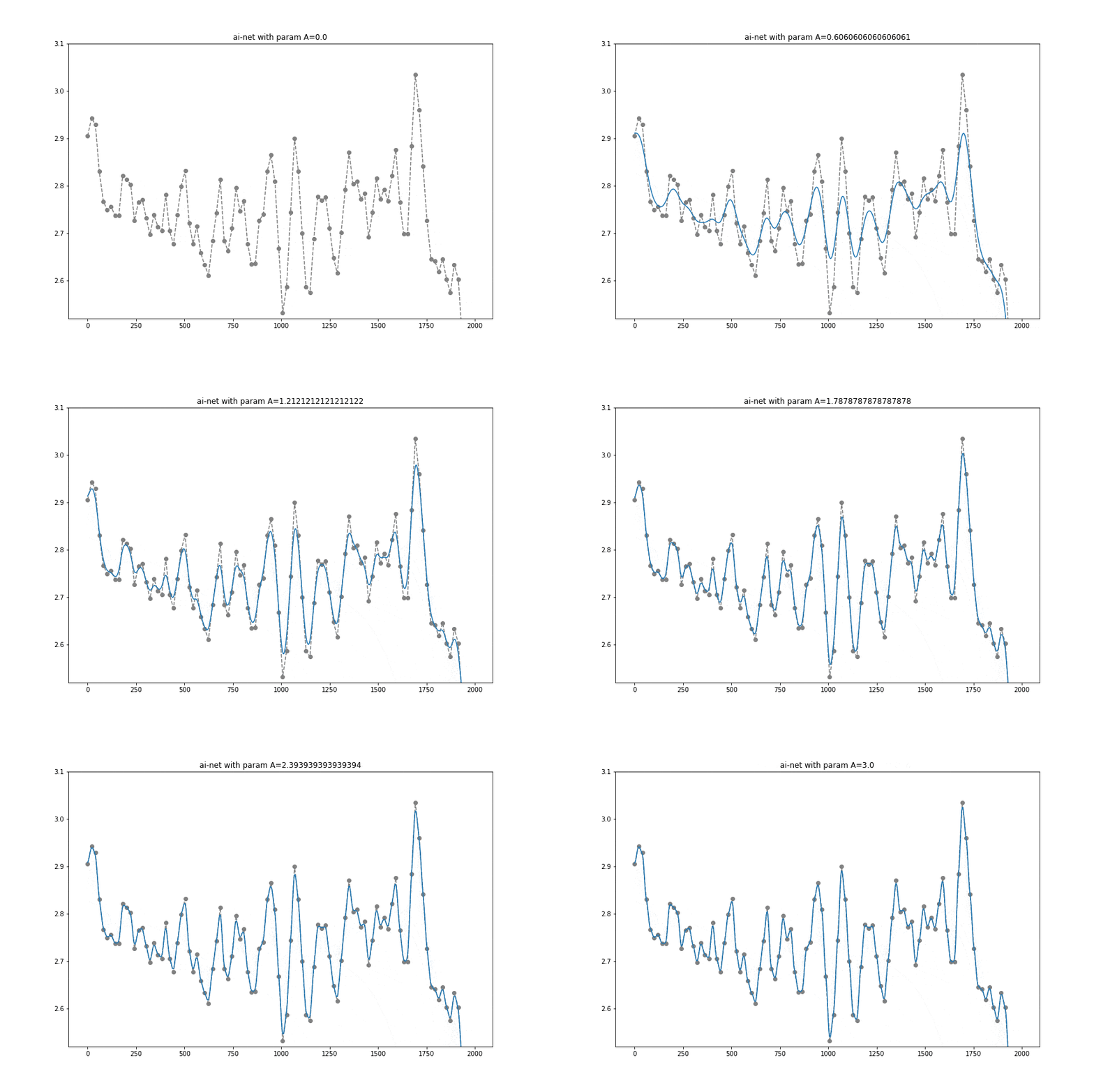
For our use case, accelerometer data at any sampling rate will go into a tflite model where it will be turned into evenly sampled (to 10Hz) and slightly smoothed values. It turns out that for the Transport Classification problem, having a higher sampling rate than 10Hz, does not lead to accuracy gain. We have empirically shown that that can replace a normalizer that usually consists of an interpolator, low-pass filter, and resampler. That's really a neat use of a simple diff, relu activation, and matrix multiplication.
Step 2. Embedding
Now, when we have cleaned up and resampled the accelerometer signal we want to construct an embedding that captures relevant features for transport classification and is not sensitive to phone rotations.
To achieve that we will use training data obtained by internally labeling thousands of trips. While running the labeling initiative we have focused on two levels of granularity which we called sensor- and trip- level. For example on the sensor level, it makes sense to have idles and phone handlings, yet these should be ignored in the next step when we move towards the final transport mode classification.

For the sensor-level model, we feed 18s sensor windows resampled to 10Hz using approximate interpolation. We trained a classifier based on InceptionTime architecture (InceptionTime: Finding AlexNet for Time Series Classification, 2019, Hassan Ismail Fawaz, Benjamin Lucas, et. al., arxiv) to distinguish between various transport modes, idles and phone handling events.
The Inception architecture is a smart improvement over the standard convolutional neural network. While the latter uses a fixed sequence of trainable filters of predefined sizes to extract information on an increasing spatial or temporal scale, an inception network has the flexibility to learn the optimal combination and sequence of applicable filter sizes themselves, thus increasing the representational power of the network.
The network is essentially composed of four identical blocks and a single residual skip connection directly from the input. In fact, these blocks are called “inception blocks” in literature. Because in a way they can be looked at like nested networks within the full network.
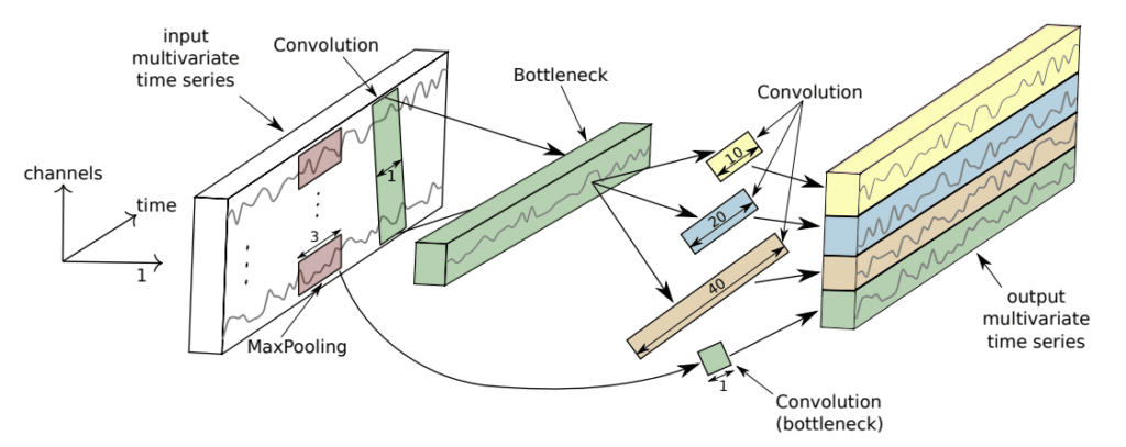
Within each inception block, the input is mapped through a bottleneck layer (size 1 kernel without bias) to three separate 1D convolution layers, with sizes along the time dimension of 10, 20 and 40 (to capture different timescales). The same input is passed through max-pooling to an additional convolutional layer which is supposed to capture features from a downsampled signal. The output is batch normalized and passed through an activation function. Eventually, the sum of the last inception block output and the residual connection is passed through global average pooling to remove the time dimension for classification.
When implementing the InceptionTime architecture, a number of changes have been made to the original architecture presented in the paper:
- The convolutional layer after MaxPool inside the inception block has kernel size 10 instead of 1 (worth ~3% accuracy)
- All convolutional layers have ReLU activation instead of linear (worth ~1% accuracy)
- Non-bottleneck convolutional layers have biases applied to them (worth ~2% accuracy)
We skip windows that have no energy and apply augmentation techniques to alleviate sensitivity to rotations and possible device fingerprinting, thereby preventing the model from overfitting particular device noise. For the training procedure, we used MLflow and AWS spot instances. It took roughly a day to train the model on a decent GPU instance.
Using this architecture, we are able to achieve ~87% accuracy on the sensor window classification, thus beating our current on-device sensor-only Transport Classifier, which achieves 84% accuracy. In the next step, we ditch the final model layers and use fixed weights to get an embedding of size 8 for each window.
To harness the power of high amounts of unlabeled data and to avoid having a two-step labeling procedure, we are currently exploring options to use unsupervised and semi-supervised learning approaches to train an embedding model.
Step 3. Trip classifier
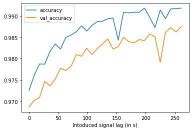
If we assume that we feed the whole trip and aim to receive segmentation at once we could use a bidirectional LSTM or similar model, but in reality, we want to achieve near real-time classifications. The goal is to find the sweet spot between accuracy and usability that we can achieve by improving response time. After running multiple experiments we found out that by introducing a lag of 3 minutes we sacrifice only 1-2% inaccuracy.
We ended up using a U-time like architecture (U-Time: A Fully Convolutional Network for Time Series Segmentation Applied to Sleep Staging, 2019, Mathias Persev, et. al., arxiv) on embeddings received from 31 windows (each represents 18s) and returning classifications at the 21st position (corresponding to a 3-minute lag). There are other papers that use U-Net in a similar domain, for example, Human Activity Recognition Based on Motion Sensor Using U-Net (2019, Yong Zhang, et.al., ieee). The main change compared to the original is that we have ditched the use of dilations and ended up using only two layers with elu activations.
A U-net architecture is in essence convolutional too, yet it enables the segmentation of the input data rather than just assigning a single class to the set as a whole. This is achieved by first doing the pixel level (or time window level, in our case) classification, which partitions input data into a set of classified blocks. The change of class in neighboring blocks thus signifies a boundary, which in our case is a change of transport mode.
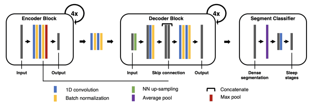
Actually, we enrich the input embeddings by appending data from GPS fixes (speed, accuracy) and various GIS features, such as distances to the nearest bus route, bus stop, or railway, computed for the given coordinates.

Did you know that Keras allows you to feed models into the TimeDistributed layer ?? Ideally, we could have trained the embedding and classifier in one go, but the required run-time exploded, thus we ended up using a two-step training process.

Step 4. Deploying on Edge
To run the model on device we decided to go with tflite. Since we will use the same runtime for various ML components our design is quite flexible and resembles the Von Neuman computer definition - new inputs and memory (state) come in and tflite outputs prediction and a new state.

In the case of our Transport Classifier, we store an embedding of the last 30 windows in the state, so that, given new sensor data, we can construct an embedding using InceptionTime and pass concatenated embeddings to U-Time.
So, at trip start our SDK collects an 18s accelerometer window and the latest GPS fix and passes those together with a dummy state (filled with -1s) to the tflite model. It receives a classification of -1 (for the first 3 minutes) and an updated state. In the next step, the SDK is responsible for feeding the new sensor window and the previous state to the model. Note, that since our model lags by 3 minutes, we have used a padded training approach. We keep calling the model for 3 minutes (by feeding padding values) after the trip ends to receive all classifications.
You might be wondering about the battery impact compared to running models on the cloud. Interestingly enough, running the model on-device consumes the same (and in some cases even less) amount of power. The main reason is that we don’t need to send high volumes of data to the backend, thus saving lots of traffic.
Performance
When using only accelerometer data with speed and accuracy from GPS fixes and evaluating on a validation set (consisting of users never seen by the model during training) we reach 91% overall accuracy (for IDLE, WALKING, RUNNING, BIKING, RAIL, VEHICLE). We are able to identify RUNNING, BIKING and VEHICLE with accuracy >95%. Note, that using only sensor signal it is nearly impossible to tell a difference between CAR and BUS, thus these classes are merged into a single class - VEHICLE.
Including GIS features (distances to the nearest bus route, bus stop, railway, etc.) that can be computed on device by preserving privacy and requesting only map tiles, we can make a separation between CAR and BUS and also distinguish TRAIN from TRAM/METRO keeping overall accuracy at ~90%.
To give a sense of how well it performs on individual trips let’s inspect some cases. In Figure 11, you can see three individual trips and predicted probability. It is displayed on top revealing that our predictions are stable over the trip.
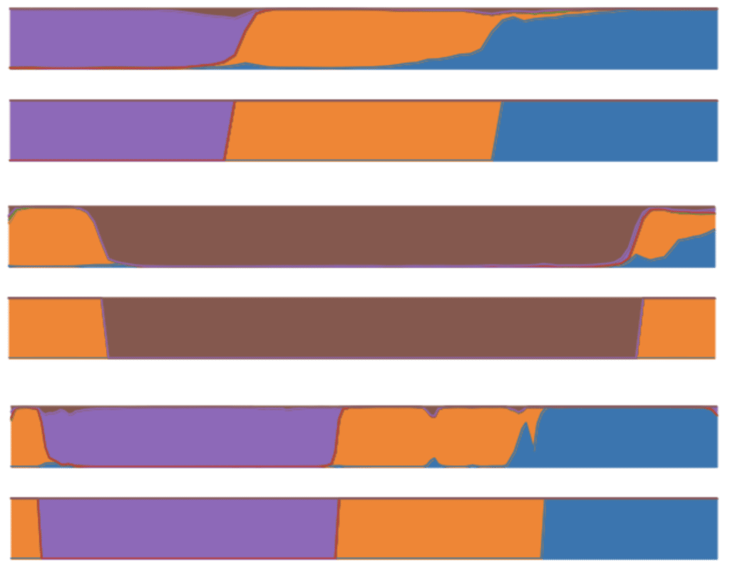
is displayed on the top and the actual transport mode on the bottom (violet - rail, orange - walking, blue - car, brown - running).
In the end, we are able to arrive at a stable prediction that prevents flip-flops and as mentioned above has a 3 minutes response time, enabling us to use it in more diverse applications than available offline solutions.
Conclusions
Having a robust and reliable Transport Classifier allows us to develop use cases in many different verticals. To mention a few we can provide mobility insights, fleet tracking, driving behavior modeling and even lifestyle coaching. Running fully on device we preserve user privacy and having a near real-time component opens up new possibilities - hyper-personalization, reacting to transport change, etc.
We are constantly improving our state of the art models. We use unsupervised and semi-supervised approaches and we are exploring opportunities to add more transport modes and functionalities on-device. In the next couple of months we plan to bring 2-wheeler support on-device, thus stay tuned.


